CONCORDIA UNIVERSITY
|
|
Dynamic Range and Stability of NR-IQA
Developed
by Meisam Rakhshanfar and Maria A. Amer
Abstract
There are some applications where the quality
measurement is used as a relative number comparison. In such applications, the relative values of measured quality are compared to
detect a quality change. Thus, we consider two properties to evaluate the NR-IQA performance: dynamic
range and stability. NR-IQA can better highlight the changes in the quality when it has a higher
dynamic range. Let us assume Idist is a low-quality noisy or blurred image and Iopt is a high qiality optimal image or the ground-truth.
NR-IQA with a high dynamic range gives results such that
Q (Iopt) >> Q (Idist).
This feature provides us the ability to detect a major quality difference by
comparing measured quality values. We propose the ratio of the highest quality
to a defined degraded image (noisy or blurred) to measure the dynamic range
DR as in,
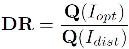 (1)
(1)
Higher values of DR show a better contrast between high and low quality inputs. NR-IQA can be designed to have a very high DR. This can be done for instance by suppressing lower values of Q(.) and magnifying the higher values. However, increasing the DR may have the downside of decreasing the stability and increasing the sensitivity. To measure stability, let us assume a random process (such as AWGN) creates different images It from a ground-truth with (almost) same quality (e.g., same distortion type with same PSNR). The NR-IQA also should give close results with a relatively small variation. If the number of random samples is large, the normalized standard deviation can be used to measure stability ST as in,
 (2)
(2)
(1) Higher values of DR show a better contrast between high and low quality inputs. NR-IQA can be designed to have a very high DR. This can be done for instance by suppressing lower values of Q(.) and magnifying the higher values. However, increasing the DR may have the downside of decreasing the stability and increasing the sensitivity. To measure stability, let us assume a random process (such as AWGN) creates different images It from a ground-truth with (almost) same quality (e.g., same distortion type with same PSNR). The NR-IQA also should give close results with a relatively small variation. If the number of random samples is large, the normalized standard deviation can be used to measure stability ST as in,
(2) Numerical Results
For a relative quality comparison, dynamic range DR and stability
ST can be considered. Higher dynamic range provides a more
contrast between low and high quality images which is useful in detection of
significant quality changes. A NR-IQA should also be stable by providing similar
results when both nature and amount of degradation are similar. We used (1) and
(2) to find the dynamic range and stability.
To create low-quality images we degraded images using AWGN with standard deviation (σa = 10)
and 5 × 5 Gaussian blur with sigma of 1 and measured the DR under
noise and DR under blur.
Table 1 compares the dynamic range of all methods. Our method
provides high dynamic range in noisy and blurry conditions.
We used (2) to test the stability. We generated 10 different
noisy images (It, t ∈ {1:10}) with same PSNR using AWGN with σa
= 10, and we calculated the QI using all methods.
Table 2 compares the normalized standard deviation of QI
and the average. The proposed method provides stable estimates having high DR as in Table 1.
1. The following experiments show average DR for 10 selected images from TID2008, Peppers, and Barbara using two types of distortions.
| BRISQUE | CPBD | JNB | LPC | S3 | BIQI | MetricQ | SDQI | |
|---|---|---|---|---|---|---|---|---|
| DR AWGN |
1.72 | 0.83 | 0.79 | 1.00 | 0.93 | 1.36 | 1.49 | 1.67 |
| DR G-Blur |
1.47 | 2.36 | 1.76 | 1.12 | 7.93 | 1.12 | 1.42 | 1.48 |
2. Normalized standard deviation (ST) of SDQI using 10 noisy samples with same PSNR (28.1dB).
| BRISQUE | CPBD | JNB | LPC | S3 | BIQI | MetricQ | SDQI | |
|---|---|---|---|---|---|---|---|---|
| Barbara | 2.50 | 0.16 | 0.47 | 0.23 | 0.38 | 0.34 | 0.28 | 0.41 |
| Kodim05 | 0.58 | 0.15 | 0.82 | 0.14 | 0.35 | 0.36 | 0.41 | 0.33 |
| Kodim06 | 1.16 | 0.20 | 0.89 | 0.23 | 0.27 | 0.33 | 0.33 | 0.50 |
| Kodim07 | 1.02 | 0.19 | 0.79 | 0.14 | 0.48 | 0.29 | 0.38 | 0.23 |
| Kodim10 | 1.23 | 0.18 | 0.83 | 0.18 | 0.22 | 0.20 | 0.70 | 0.61 |
| Kodim17 | 1.43 | 0.19 | 1.21 | 0.19 | 0.41 | 0.21 | 0.64 | 0.42 |
| Peppers | 0.99 | 0.21 | 1.34 | 0.31 | 0.39 | 0.69 | 0.37 | 0.52 |
| Average | 1.27 | 0.18 | 0.91 | 0.20 | 0.36 | 0.35 | 0.44 | 0.43 |