The GO_3D Code for Indoor Propagation
Professor Christopher W. Trueman
Electromagnetic Compatibility Laboratory
Revised
Abstract- These notes present program GO_3D for computing the fields of a transmitter in an indoor environment using geometrical optics. The program uses a “image tree” data structure to construct the images needed to compute all the rays carrying fields above a preset “threshold” value, no matter how many reflections are needed. The input command structure of the program is presented. An application of the GO_3D program to a small room adjacent to a long corridor is presented.
1 Introduction
Propagation of radio waves in an indoor environment has become important because of the widespread use of wireless technology. Cellular telephones are frequently used indoors and must communicate with base stations located on nearby buildings or towers. Walkie-talkies are used by security guards. Wireless LANs are used to network computers and printers without the need for expensive, messy wiring that is costly to reconfigure. For adequate communication, the signal strength at the receiver due to a transmitter elsewhere in the building must exceed a minimum value. Conversely, electromagnetic interference or EMI can result if the signal strength of a transmitter exceeds the maximum permissible field strength or “immunity” of another device. EMI is of particular concern in hospital environments where medical equipment may malfunction, with grave consequences, if the signal strength of a cellular phone or walkie-talkie is larger than the 3 V/m immunity. Thus, for adequate communication, signals are required to exceed a minimum value, but to prevent EMI signals must not exceed a specified maximum.
Wireless design in a indoor environment sometimes uses a simple-minded approach to propagation. In this approach, the signal strength of the transmitter is modeled as
![]()
where ![]() is the field strength
of the transmitter in free space at one meter distance; and
is the field strength
of the transmitter in free space at one meter distance; and ![]() is the geometrical
distance. Exponent
is the geometrical
distance. Exponent ![]() is unity in free
space, and is larger than 1 in an indoor environment. Ref. [1] tabulates values of
is unity in free
space, and is larger than 1 in an indoor environment. Ref. [1] tabulates values of ![]() recommended for
various indoor environments. Also, each
time the ray from the source to the transmitter penetrates a wall, the signal
strength is reduced[2] by attenuation factor
recommended for
various indoor environments. Also, each
time the ray from the source to the transmitter penetrates a wall, the signal
strength is reduced[2] by attenuation factor ![]() . This model has the
merit of extreme simplicity and can be used to make useful maps of the signal
strength expected throughout the floor of a building due to a transmitter in a
specified location, to ensure adequate communication.
. This model has the
merit of extreme simplicity and can be used to make useful maps of the signal
strength expected throughout the floor of a building due to a transmitter in a
specified location, to ensure adequate communication.
Where
more detailed, realistic maps of the signal strength in an indoor environment
are needed, geometrical optics (GO) is often used[3,4,5]. The GO model traces rays from the transmitter
location (Tx) to the receiver location (Rx).
If there is a line-of-sight path, there is a “direct” ray carrying the
field strength of the transmitter in free space, fully accounting for its
directional properties and the polarization of the wave. A ray can reflect from a wall surface en route
from the transmitter to the observer.
The angle of incidence and of reflection must obey Snell’s Law[3] which
determines a unique reflection point on the wall surface between the Tx and the
Rx. The field strength of the reflected
wave depends on the angle of incidence to the normal, on the polarization of
the wave, on the wall construction and on the frequency. Usually, the interaction is treated as
“local”, meaning that the incoming and reflected waves are considered to be
plane waves, and so plane wave reflection coefficients are used. Plane wave reflection and transmission
coefficients are available for homogeneous panels of a given material and thickness[3] and for panels which are
constructed of layers of material, each with given electrical properties and
thickness[6]. These can be used to model
walls built of homogeneous layers.
Coupling paths from the transmitter to the receiver may involve two,
three or many reflections from the walls.
In a practical GO computation, only a limited number of reflections can
be accounted for, and choosing whether 3, 10 or 20 reflections is enough is an
important issue. The wave from the
transmitter may penetrate a wall, which reduces its field strength by a
transmission coefficient dependent on the frequency, polarization and wall
construction. The field arriving at the
receiver is the sum of the fields associated with all the rays that arrive
there. In an indoor environment, waves
usually arrive from many different directions, having followed ray paths with a
wide range of path lengths. Still, GO
can find a vector sum of all the fields, and so find the vector components ![]() ,
, ![]() and
and ![]() of the field at any
given location.
of the field at any
given location.
Two
approaches to computing fields by geometrical optics have been used. In the “shooting and bouncing rays”
method[5], a sphere surrounding the transmitter is divided into ![]() patches and a ray is
launched though the center of each patch.
Thus each ray accounts for the energy radiated from the source over a
solid angle of
patches and a ray is
launched though the center of each patch.
Thus each ray accounts for the energy radiated from the source over a
solid angle of ![]() steradians. As the distance from the source increases,
the cross-sectional area associated with the ray increases. When the ray passes an observer, if the
observer lies within this area, the ray contributes field to the observer. When
the ray encounters a wall, two rays are created that must be tracked. The transmitted ray’s field strength is
reduced by the transmission coefficient.
The reflected ray’s field is reduced by the reflection coefficient. Each these rays is traced through further
reflections, giving rise to further rays, and every ray eventually exits the
problem space. Shooting and bouncing
computer codes usually discard rays after a fixed number of reflections, or
when the field strength associated with the ray falls below a threshold value.
steradians. As the distance from the source increases,
the cross-sectional area associated with the ray increases. When the ray passes an observer, if the
observer lies within this area, the ray contributes field to the observer. When
the ray encounters a wall, two rays are created that must be tracked. The transmitted ray’s field strength is
reduced by the transmission coefficient.
The reflected ray’s field is reduced by the reflection coefficient. Each these rays is traced through further
reflections, giving rise to further rays, and every ray eventually exits the
problem space. Shooting and bouncing
computer codes usually discard rays after a fixed number of reflections, or
when the field strength associated with the ray falls below a threshold value.
The
second approach to GO computations uses the method of images[3]. The transmitter gives rise to an image in
each of the wall panels, and in the floor and the ceiling. This set of “first level” images is
sufficient to compute all the rays that have one reflection in traveling from
the Tx to the Rx. Each image source
itself has an image in every wall panel; this set of “second level” images
permits the computation of ray paths having two reflections. Similarly, every 2nd level image
has a 3rd level image in each wall panel. Constructing images to ![]() levels permits the
computation of ray paths with
levels permits the
computation of ray paths with ![]() reflections. The set of images form a “tree” data structure
and it is convenient to create and store an “image tree”[4]. The strength of the field associated with a
ray after
reflections. The set of images form a “tree” data structure
and it is convenient to create and store an “image tree”[4]. The strength of the field associated with a
ray after ![]() reflections is reduced
by the product of
reflections is reduced
by the product of ![]() reflection
coefficients; so it is argued that fields of rays having been reflected more
than say 3 or 10 or 20 times will be negligible, and so the “image tree” can be
truncated after 3 or 10 or 20 levels.
Usually the set of images is constructed individually for each observer
location, as many image sources can be immediately discarded because they
cannot give rise to a reflected ray for that observer.
reflection
coefficients; so it is argued that fields of rays having been reflected more
than say 3 or 10 or 20 times will be negligible, and so the “image tree” can be
truncated after 3 or 10 or 20 levels.
Usually the set of images is constructed individually for each observer
location, as many image sources can be immediately discarded because they
cannot give rise to a reflected ray for that observer.
Geometrical optics has the disadvantage that the field strength contains discontinuities that arise when rays abruptly disappear. Thus as an observer moves past a corner, the “direct” ray path from Tx to Rx can be interrupted by the corner, and the direct ray vanishes. The field abruptly drops by the value associated with the direct ray. Uniform Diffraction Theory[3] smoothes the field by accounting for the diffracted field of the edge. This adds very considerable complication to the calculation but has been included in some formulations[4].
This
paper presents a three-dimensional geometrical optics program for indoor
propagation called “GO_3D”. The user
defines the floor plan using layered wall construction by specifying the
locations of the wall panels. The
transmitter location and directional patterns are defined. Points at which GO_3D must find the field are
called “receivers”. There can be just one receiver, or receivers spaced along a
line or evenly spaced on a grid. GO_3D
uses an image tree method in which the tree is constructed once at the outset
of the problem, and is valid for all observers. The same image tree is used to
computed the reflected and transmitted rays for all observers, although many of
the image sources will not give rise to rays at one individual observer
location. GO_3D requires the user to
specify a threshold value, and all the rays with field strengths greater than
the “cutoff” field strength are included in the computation. GO_3D uses a fully three-dimensional, vector
calculation accounting for the magnitude and phase of both vector field
components associated with each ray. For
a single observer, the program creates graphics showing the ray paths, and a
file giving the field strength and path length for each ray. For lines of receivers, the field strengths ![]() ,
, ![]()
![]() and
and ![]() can be graphed as a function of distance. For grids of receivers, each field component
can be graphed as a contour map. A User’s Guide is available on-line[7].
can be graphed as a function of distance. For grids of receivers, each field component
can be graphed as a contour map. A User’s Guide is available on-line[7].

Figure 1 A system of three walls and a transmitter (Tx). The first two levels of images are shown.

Figure 2 The image tree showing the transmitter and three levels of images.
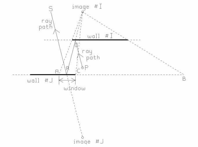
Figure 3 An image source I and its image J in wall #J.
2 The Ray Tracing Algorithm
This section briefly describes the ray tracing method used by the
GO_3D computer code. Fig. 1 illustrates
the construction of the set of images for a transmitter “Tx” and a system of
three walls, leading to the tree structure of images shown in Fig. 2. The 1st level of the tree contains
the image of the transmitter in each of the three walls, labeled as sources
(1,1), (1,2) and (1,3). Also, the source
generating the image has been identified as “Tx” in each case, and the wall
identified as “w1” for wall #1, etc.
Images at level i in the tree
are numbered sequentially, j=1,2,3,
so each image is identified by an ordered pair ![]() . For our system of
three walls, these three 1st level image sources are sufficient to
compute all ray paths having one reflection from the transmitter to the
observer. The 2nd level of
the tree contains the image of each 1st level source in each wall,
except the wall that created the 1st level image. Image source (1,1) is an image in wall #1,
and generates 2nd level image (2,1) in wall #2, and image (2,2) in
wall #3. Imaging sources (1,2) and (1,3)
gives 6 images at the second level, as shown in Fig. 1. This is sufficient to compute all ray paths
with one reflection or with two reflections from the transmitter to the
observer. The third level has the image
of six 2nd level sources in two walls, for a total of twelve
images. The image sources are
conveniently arranged in the tree data structure of Figure 2. Note that the
image tree is correct for any
location of the observer, so the same
image tree can be used to find the field for all possible observers.
. For our system of
three walls, these three 1st level image sources are sufficient to
compute all ray paths having one reflection from the transmitter to the
observer. The 2nd level of
the tree contains the image of each 1st level source in each wall,
except the wall that created the 1st level image. Image source (1,1) is an image in wall #1,
and generates 2nd level image (2,1) in wall #2, and image (2,2) in
wall #3. Imaging sources (1,2) and (1,3)
gives 6 images at the second level, as shown in Fig. 1. This is sufficient to compute all ray paths
with one reflection or with two reflections from the transmitter to the
observer. The third level has the image
of six 2nd level sources in two walls, for a total of twelve
images. The image sources are
conveniently arranged in the tree data structure of Figure 2. Note that the
image tree is correct for any
location of the observer, so the same
image tree can be used to find the field for all possible observers.
2.1 The Image’s Window
With ![]() walls, there are
walls, there are ![]() images at the 1st
level,
images at the 1st
level, ![]() images at the 2nd level,
images at the 2nd level, ![]() images at the 3rd
level, and so forth, and the number of image sources at each level grows
rapidly. However, some image sources can
be discarded immediately because the walls are not infinite planes. Consider the configuration in Fig. 3, where
image source I is an image in wall #I, and at the next level, image source J is
an image of source I in wall #J. The
projection of wall #I from image source I onto wall #J is segment AB in the
plane of wall #J. In three dimensions
this is an area. The portion of AB that
lies within the physical area of wall #J is segment AC, and is called the
“window” associated with image source #J in wall #J. A ray from image source #J must pass through
the “window” to be physically possible.
Thus the ray from some source at P, reflected at Q from wall #I,
reflected at R from wall #J, and reaching an observer at S, is physically
possible. If the segment AB on the plane
of wall #J does not intersect any part of wall #J, then the window is of zero
extent and image source J can be discarded as the image tree is
constructed. This eliminates a great
many image sources from the tree.
images at the 3rd
level, and so forth, and the number of image sources at each level grows
rapidly. However, some image sources can
be discarded immediately because the walls are not infinite planes. Consider the configuration in Fig. 3, where
image source I is an image in wall #I, and at the next level, image source J is
an image of source I in wall #J. The
projection of wall #I from image source I onto wall #J is segment AB in the
plane of wall #J. In three dimensions
this is an area. The portion of AB that
lies within the physical area of wall #J is segment AC, and is called the
“window” associated with image source #J in wall #J. A ray from image source #J must pass through
the “window” to be physically possible.
Thus the ray from some source at P, reflected at Q from wall #I,
reflected at R from wall #J, and reaching an observer at S, is physically
possible. If the segment AB on the plane
of wall #J does not intersect any part of wall #J, then the window is of zero
extent and image source J can be discarded as the image tree is
constructed. This eliminates a great
many image sources from the tree.
In carrying out ray tracing for an observer at S, first a ray is traced from image J to S. The intersection of this ray with the “window” of image source J, i.e. line segment AC, must lie within the window, or else the ray can be discarded. If the ray is possible, then the ray is traced back to image source I, and the intersection of the IJ ray with the plane of wall #I must line within the “window” of image source I(not shown on the figure). If it does then I can be joined with the source, P, and a two-reflection ray path has been found. Thus each entry in the image tree contains the 3D coordinates of an image source, and the associated window. The image source looks out on the world through the window, meaning that rays from the image source must pass through the window to be physically possible.
The concept of “window” eliminates many images from the tree but is not sufficient as a stopping criterion. The GO_3D code uses a minimum field strength associated with an image source to terminate the image tree, as explained in the following.
2.2 The Threshold
Ideally a geometrical optics analysis should track each ray through many reflections and transmissions until it exits from the problem space. But at each reflection, there is a transmitted ray, which must also be traced until it exits from the problem space. The computation quickly becomes very time-consuming and hence expensive. So geometrical optics computer codes must decide to discard each ray at some point. For most wall materials, the field strength associated with the ray is substantially reduced either when the ray penetrates a wall or when the ray reflects from a wall. After a number of reflections the field strength associated with a ray might be expected to be negligible, and the ray can discarded, and not tracked any further. Many geometrical optics codes require that the user specify, a priori, the maximum number of reflections that the code will track. The implicit assumption is that after this many reflections the field strength associated with any ray is negligible. But this can be misleading. For example, for near-grazing incidence, the reflection coefficient approaches unity for any type of wall construction. Obviously, if a ray undergoes say four reflections at near grazing incidence, the reflection coefficient at each reflection is nearly unity and the field is not reduced by reflection. The ray still carries a significant amount of power and should not be discarded.
The
GO_3D code uses a different criterion for discarding a ray. Each ray is traced through as many
reflections as required to reduce its estimated field strength to less than a
“cutoff” field strength ![]() . If the transmitter
radiates
. If the transmitter
radiates ![]() watts of power then
the “isotropic level” field strength is
watts of power then
the “isotropic level” field strength is
![]()
The user specifies the threshold ![]() to the GO_3D code in
dB below the isotropic level. The cutoff
field strength is then
to the GO_3D code in
dB below the isotropic level. The cutoff
field strength is then
![]()
For a 600 mW
source, the isotopic level is 5.998 V/m, or about 6 V/m. A threshold of ![]() 20 dB with a 600 mW source instructs the code to discard
image sources having fields less than
20 dB with a 600 mW source instructs the code to discard
image sources having fields less than ![]() 0.6 V/m. An image
source is included in the calculation if the largest field strength it can give
rise to, for any observer, is greater than or equal to the “cutoff” field
strength. The code will construct the
image tree to as many levels as needed to include all such sources.
0.6 V/m. An image
source is included in the calculation if the largest field strength it can give
rise to, for any observer, is greater than or equal to the “cutoff” field
strength. The code will construct the
image tree to as many levels as needed to include all such sources.
In practice, the GO_3D code constructs the “image tree” once, after the input geometry file has been read, and then uses the same image tree for all the receiver positions. Thus, the location of an observer cannot be a criterion for whether an image should or should not be included in the image tree. The field an image source gives rise to is of the form
![]()
where ![]() is the strength of the
transmitter in the direction associated with the image source,
is the strength of the
transmitter in the direction associated with the image source, ![]() is the net attenuation
along the path including the reflection loss when the ray is reflected from
walls and the transmission loss when the ray penetrates walls. Distance
is the net attenuation
along the path including the reflection loss when the ray is reflected from
walls and the transmission loss when the ray penetrates walls. Distance ![]() is the minimum
possible distance from the source to the observer, hence the observer location
that is closest to the image source is used.
To decide whether to include or discard an image, the GO_3D code uses
is the minimum
possible distance from the source to the observer, hence the observer location
that is closest to the image source is used.
To decide whether to include or discard an image, the GO_3D code uses ![]() , the source’s isotropic level, and assumes no loss of
amplitude due to transmission or reflection,
, the source’s isotropic level, and assumes no loss of
amplitude due to transmission or reflection, ![]() , which is the worst case.
An image is retained if
, which is the worst case.
An image is retained if
![]()
or
equivalently if ![]() where the cutoff
distance is
where the cutoff
distance is ![]() . Thus, the decision
of whether to retain or discard an image in the image tree is based simply on
the nearest possible distance from the image source to an observer.
. Thus, the decision
of whether to retain or discard an image in the image tree is based simply on
the nearest possible distance from the image source to an observer.
Figure 4 Tracing a ray using the image tree.
2.3 Tracing Rays to an Observer
In a typical calculation, the field is required at many points along
a line, or at many points covering a rectangular grid. Each such point is a “receiver”. The image tree is constructed once, and then
used to find the field at all of the receivers.
Consider the image tree of Fig. 2, with three levels. To trace all possible rays the program must
start with each individual image source, and try to trace a ray from the
receiver, via that source, back through the image tree to the transmitter. The ray-tracing method for image (3,3) is
shown in Figure 4. Join the receiver Rx
to image (3,3) with a ray and find intersection P3. If P3 does not lie within the “window” of
image (3,3) discard the ray path and move on to the next image source. But if P3 lies within the window, then join
P3 to the “parent” image in the tree of Figure 2, namely image (2,2). If reflection point P2 lines within the
window of image (2,2), then join P2 to the “parent” in the tree, which is image
(1,1), to find P1. If P1 lies in the
window of image (1,1), then join P1 to the parent, which is the
transmitter. Then path Tx to P1 to P2 to
P3 to Rx is a ray path. To find the
field at Rx, find the vector components of the transmitter’s field along path
Tx to P1, accounting for the directional antenna patterns and polarization of
the transmitter. The dyadic reflection
coefficient at P1 accounts for the reflection coefficient for the “parallel”
and “perpendicular” component of the field at the reflection point, and for the
angle of incidence form the normal. Use
the dyadic reflection coefficient for wall #1 to reflect the field at P1 and so
obtain the vector components of the field along the P1 to P2 path. Similarly,
the dyadic reflection coefficients are used at P2 and P3, and finally the ray
is “propagated” to the receiver, Rx. The
result is the magnitude and phase of the three vector components of the field, ![]() ,
, ![]() and
and ![]() , at the receiver on a three-reflection path using image
source (3,3). The process must be
repeated for all the image sources at level 3; this finds all possible
three-reflection paths. Then look for
two-reflection paths starting with image source (2,1), considering all 2nd
level image sources in turn. This finds all possible two-reflection paths. The consider each 1st level image
in turn to find one reflection paths.
Finally the direct path from the source is found. Adding the fields due to all the rays that
are found obtains the net field strength at the observer.
, at the receiver on a three-reflection path using image
source (3,3). The process must be
repeated for all the image sources at level 3; this finds all possible
three-reflection paths. Then look for
two-reflection paths starting with image source (2,1), considering all 2nd
level image sources in turn. This finds all possible two-reflection paths. The consider each 1st level image
in turn to find one reflection paths.
Finally the direct path from the source is found. Adding the fields due to all the rays that
are found obtains the net field strength at the observer.
The search for ray paths using the image tree is repeated for each “receiver” that the user has specified.
3 The GO_3D Input File
The user of the GO_3D program must prepare a text file, with extension “go3”, which describes the construction and location of the walls, gives the frequency and location of the transmitter, and defines the position of “receivers” where the field must be calculated. The program uses a descriptive input “language” based on the commands in Table 1. The program’s command interpreter uses the keyword at the beginning of each line to identify each “command”. Any line beginning with capital-C is a “comment line” and is ignored; users are encouraged to annotate their input files liberally for later reference. A complete description of the input commands including a comprehensive example can be found in the GO_3D User’s Guide[7].
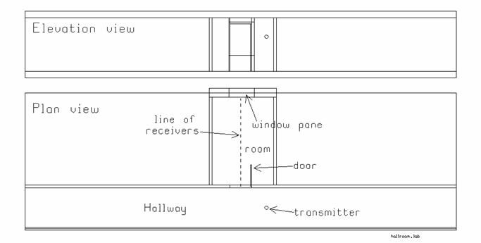
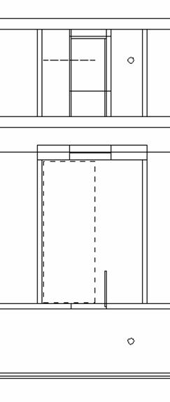
Figure 5 The hallway with a side room.
The use of GO_3D will be illustrated with the problem in Figure 5, which shows a floor plan or xy plane view in the lower part of the figure and an elevation or xz plane view in the upper part. The floor plan consists of a corridor 40 m long and about 2 m wide. There is a transmitter in the corridor that represents an 850 MHz cell phone radiating 600 mW. The cell phone’s radiation patterns will be modeled with those of a vertical, half-wave dipole, at a height of 1.6 m above the floor. One room off the corridor is included in this simple floor plan. The doorway is 1 m wide and is near the transmitter. The door is wood, 10 cm thick, and is in the “open” position. The room measures about 3 by 4 m. The problem is to determine the field strength along the path indicated by the dashed line in Fig. 5, starting near the center of the doorway and ending near the window.
3.1 Wall Materials and Construction
The construction of the walls is specified to the GO_3D program first by using the keyword “MATERIAL” in Table 1 to define materials by giving each a name and values for the electrical parameters. Table 1 defines a material named “Space” with the electrical properties of free space, and materials called “Concrete” and “Brick”. Next, wall constructions are defined with “WALL_TYPE” by giving each a name and specifying the material and thickness of the various layers. Thus a “ConcreteWall” has a single layer (hence is “SOLID”), is made of the material previously named “Concrete”, and is 42 cm thick. A “SheetrockWall” has three layers (hence is “LAYERED”). The layers are 1 cm of the material called “Concrete” representing a sheetrock panel, 12 cm of “Space” representing an air space between the sheetrock surfaces; and a 1 cm thick “Concrete” on the other side.
3.2 The Floor Plan
To specify the location of the wall panels making up the floor plan, the geometry commands of Table 1 are used. A wall panel is defined by giving the location of two opposite corners of a rectangle in the center plane of the wall. Points in 3D space are defined with the POINT command. Each point is given a name and assigned xyz coordinates. Preparing an input file requires a floor plan of the building in which propagation is to be studied. Only the minimum number of walls should be included in the input file so that the calculation will be as rapid as possible. The locations of the central planes of the various walls are scaled from the floor plan. In Table 1, two points called “23” and “24t” are defined with the POINT command and are the bottom corner and the opposite top corner of the center plane of a wall at x=6.095, from y=-1.12,z=0. to y=0.85,z=2.48 m. Keyword “DEFINE_WALL” is used to create the wall panel by invoking the two points 23” and “24t” as the corners, and then stating that the wall construction is “SheetrockWall”, which has been defined previously. Wall panels must be parallel to the coordinate planes.
The “FLOOR” command is used to instruct the program to include a floor in the calculation, using the material “Concrete” 42 cm thick in Table 1. The floor level is z=0, by definition. The GO_3D program sets the size of the floor to fit underneath all of the wall panels. Then rays that are launched by the transmitter downward will be reflected by the floor back up into the problem. Similarly, the “CEILING” lets the user include a ceiling of a given material and thickness, at a given height above the floor. Then rays launched upward from the source, or reflected from the floor, can also be reflected by the ceiling. No wall panels are permitted to extend into the floor, below z=0, nor into the ceiling, above z=2.48 m for the ceiling of Table 1. Many real buildings have a hanging ceiling which conceals a complex array of conduits, air ducts, wiring, and pipes for plumbing. Such a ceiling does not reflect spectrally, but rather scatters the field in a complex way. A uniform, smooth ceiling is a poor model.
When the GO_3D code is run, the program creates a geometry file called PLAN.LAB, which contains a drawing of the problem in the format shown in Fig. 5. The file with extension “lab” is graphed with program “LABLNG”[8]. The LABLNG program lets the user add text strings to the floor plan such as “hallway” or “room” or “transmitter”, so that the diagram is useful for inclusion in a report. With a single observer, the file also shows the rays interconnecting the transmitter and the observer, as discussed below. With a line of observers the drawing shows the location of the line, namely the dashed line in Fig. 1. Similarly, with a grid of observers, the graph shows the location of the grid. In constructing a floor plane, it is recommended that walls be added a few at a time. GO_3D is run with no receiver positions specified. The program generates the “plan” file then exits on a “no receivers” error. The plan can be examined to verify that the new walls are correctly positioned.
3.3 The Transmitter
The user
must define the source or transmitter.
The command “FREQUENCY” is used to set the operating frequency in MHz.
The power radiated by the source in mW is set with “SOURCE_POWER”, and is 600
mW in Table 1. The location of the
source is set by defining a POINT, called “xmitter” in Table 1, and then using
the command SOURCE_LOCATION to set the defined point as the position of the
source. There are two options for
modeling the source itself. The command
“DIPOLE” defines the source to be a half-wave dipole, and gives a unit vector
parallel to the axis of the dipole. Thus
in Table 1, the dipole source is parallel to the z axis. Much more complex
sources can be imported into the problem.
For example, a realistic model of a cellular telephone handset operating
near a model of the head might be used as a source. The transmitter must then be solved by a
method such as the finite-difference time-domain method to determine the
magnitude and phase of the electric field components ![]() and
and ![]() over the surface
of the radiation sphere. This is done by
computing 21 “conical
cuts” for
over the surface
of the radiation sphere. This is done by
computing 21 “conical
cuts” for ![]() =0, 25, 37, 45, 53, 60, 66, 72, 78, 84, 90, 96, 102, 108,
114, 120, 127, 135, 143, 155 and 180 degrees, each at five degree increments in
angle
=0, 25, 37, 45, 53, 60, 66, 72, 78, 84, 90, 96, 102, 108,
114, 120, 127, 135, 143, 155 and 180 degrees, each at five degree increments in
angle ![]() . The information is stored in a file called a “solution” file or
“sol” file, and imported into GO_3D with the “IMPORTED_SOURCE” command, which
supplies the name of the file. The
User’s Guide[ref] gives the details of the “sol” file format. The “solution” file must explicitly state the
power radiated by the user’s source configuration, and then the fields in the
file are rescaled to the power level specified by the SOURCE_POWER
command. The GO_3D program uses linear
interpolation to find field values at angles
. The information is stored in a file called a “solution” file or
“sol” file, and imported into GO_3D with the “IMPORTED_SOURCE” command, which
supplies the name of the file. The
User’s Guide[ref] gives the details of the “sol” file format. The “solution” file must explicitly state the
power radiated by the user’s source configuration, and then the fields in the
file are rescaled to the power level specified by the SOURCE_POWER
command. The GO_3D program uses linear
interpolation to find field values at angles ![]() ,
,![]() between the angles explicitly contained in the “sol” file
data set.
between the angles explicitly contained in the “sol” file
data set.
3.4 The Receivers
The locations at which the field is to be computed are called “receivers”. To calculate the field at a single point, use POINT to associate the coordinates with a symbolic name such as “rcvr”, and then use the command “RCVRPOINT rcvr” to set the receiver location. This is primarily used to study the ray coupling paths between the transmitter and the desired receiver location, as discussed later in this paper.
To calculate the field strength on a line from
one point to another, the two points are defined with “POINT” commands as, say,
“rstart” and “rend”. Command “RCVRLINE
rstart rend 2.0” causes the GO_3D program to compute the field at points on a
line starting a “rstart”, proceeding towards “rend” in 2 cm steps. The program creates an output file
“RCVR.DAT” containing a table giving distance along the line, and the
magnitudes of ![]() ,
, ![]() ,
, ![]() , and the “total field
, and the “total field ![]() , defined by
, defined by
![]()
Then the field components as a function of distance from “rstart” to “rend” are readily graphed.
To
calculate the field over a rectangular grid of points, the “POINT” command is
used to define the coordinates of the corners of the rectangle, say at points
named “gridst” and “griden”. Then
“RCVRGRID gridst griden 3.5” is used to command the program to calculate the
field on a grid of points spaced 3.5 cm apart, with point “gridst” as the first
point. The plane of the grid must be
parallel to a coordinate plane. This is used to investigate the field over the
area of a room due to a transmitter in a specific location, for example. The output is a table giving the coordinates
of each point in the grid, and the value of ![]() ,
, ![]() ,
, ![]() and
and ![]() at each point.
at each point.
3.5 Program Control
The threshold field strength is specified with the “ETHRESHOLD” directive. The user supplies the value of T in decibels below the isotropic level field strength, as discussed above.
The command “RAYLISTS” causes the program to create a text file called “RAYLISTS.DAT”. This file contains a detailed list of all the rays that couple the transmitter and receiver. The geometrical coordinates of all the reflection points are given, so it is possible to trace the path of each ray through the floor plan. The length of the ray path is given, and the field strength associated with the ray at the receiver. The “RAYLISTS” command is usually used with only one receiver and a modest value for the threshold. If “RAYLISTS” is used with lines or grids of receivers, the rays for all the receivers are listed and the file can get very large.
Fields as a function of distance along a line are often graphed with program RPLOT, a general-purpose “rectangular plotter” software[9]. RPLOT can graph the RCVR.DAT file previously mentioned, it is more convenient to have the GO_3D program create an output file in “native RPLOT” format. This includes axis formatting and documentation such as the name of the “go3” input file used to create the data, and the date. Thus if the field strength along a line is requested with the RCVRLINE command, and if the command “RPLFILE” is included, then GO_3D will create output in RPLOT format.
The
field strength over an area is often graphed as a color contour map with
program CPLOT or “contour plotter”[10].
It is convenient to have GO_3D prepare the output from a RCVRGRID
command in “native CPLOT” format as a “table” file. If the command TBLFILE is included in the
input file, then the fields ![]() ,
, ![]() ,
, ![]() and
and ![]() are stored in individual “table” files, each
of which can be graphed directly with CPLOT.
are stored in individual “table” files, each
of which can be graphed directly with CPLOT.
|
Table 1 GO_3D Input Commands |
|
MATERIAL Space
1. 0. 1. MATERIAL Concrete
6.1 60.1 1. MATERIAL Brick
5.1 10. 1. MATERIAL Iron
1.0 2.E9 1000. WALL_TYPE
BrickWall SOLID Brick
14. WALL_TYPE
ConcreteWall1 SOLID Concrete 42. WALL_TYPE
SheetrockWall LAYERED 3 Concrete 1.
Space 12. Concrete 1. WALL_TYPE
ClayBlockWall LAYERED 5 Concrete 1.5
Brick 0.8 Space 9.4 Brick 0.8 Concrete 1.5 WALL_TYPE
Plaster&Wire LAYERED 3 Concrete 1.
Iron 12. Concrete 1. |
|
POINT
xmitter 3.9225 1.35 1.6 POINT 23 6.095 -1.12
0. POINT 24t 6.095 0.85
2.48 DEFINE_WALL 23 24t SheetrockWall FLOOR
Concrete 30. CEILING Concrete 30.
2.48 |
|
FREQUENCY 850. SOURCE_POWER 600. SOURCE_LOCATION xmitter DIPOLE_SOURCE 0.
0. 1. IMPORTED_SOURCE verdple.sol |
|
RCVRPOINT rcvr RCVRLINE rstart
rend 2.0 RCVRGRID gridst griden 3.5 |
|
Program Control RPLFILE |
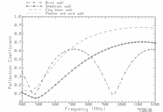
Figure 6(a) The reflection coefficient for various wall constructions as a function of frequency, for normal incidence.
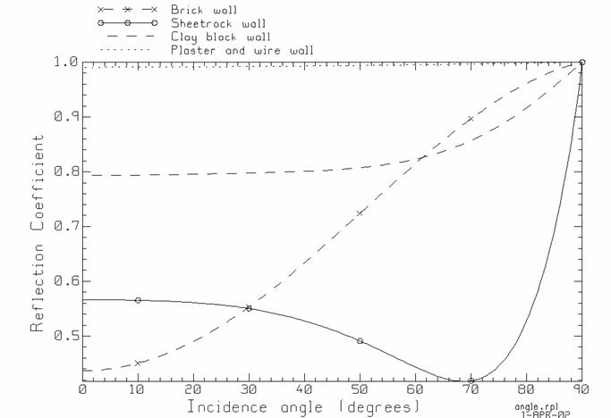
Figure 6(b) The reflection coefficient for various wall constructions at 850 MHz.
4 Reflection Coefficient for Four Wall Constructions
When the command “REFANGLE” is included in the input file, then GO_3D creates an output file for each wall construction that shows the value of the reflection coefficient for parallel and perpendicular polarization, and of the transmission coefficient for parallel and perpendicular polarization, as a function of the angle of incidence, at the operating frequency. These files are called ANGLEnn.DAT, where “nn” is the wall construction number. Thus for example the 3rd WALL_TYPE in Table 1 is “SheetrockWall” and its data would be found in ANGLE03.DAT. Program RPLOT can be used to graph the data in this file[9]. Similarly when the command “REFFREQ 400. 1200.” is included in the input file then the GO-3D program creates a file giving the reflection coefficient and the transmission coefficient as a function of frequency over the specified range, here from 400 to 1200 MHz. The data file for the 3rd WALL_TYPE is called FREQ03.DAT and can be graphed with RPLOT.
The reflection coefficient of the walls has a profound effect on the
field strength that a source generates, both in the same room or corridor, and
in adjacent rooms of the floor plan.
Four types of wall construction are defined in Table 1. The construction named “BrickWall” is a solid, 12 cm layer of brick,
with![]() mS/m at 850 MHz. A
“Sheetrock” wall consists of surface sheets of drywall 1 cm thick, separated by
a 12 cm air layer. The drywall is
represented with the electrical properties of concrete,
mS/m at 850 MHz. A
“Sheetrock” wall consists of surface sheets of drywall 1 cm thick, separated by
a 12 cm air layer. The drywall is
represented with the electrical properties of concrete, ![]() mS/m. The construction named “ClayBlockWall” models a real
wall construction using hollow clay blocks with a wall thickness of 8 mm, faced
with plaster. This is represented as a
layered structure with a 1.5 cm plaster (concrete) facing, a 0.8-cm brick wall
of the clay block, a 9.4 cm thick air space inside the clay block, the 0.8-cm
block wall and the 1.5-cm plaster facing on the other side of the wall. Some clay block walls have metal screen
embedded within the plaster. The
construction named “Plaster&Wire” models a 1 cm thick plaster (concrete)
facing backed by a very highly conducting metal layer. Such walls are almost perfectly
reflecting.
mS/m. The construction named “ClayBlockWall” models a real
wall construction using hollow clay blocks with a wall thickness of 8 mm, faced
with plaster. This is represented as a
layered structure with a 1.5 cm plaster (concrete) facing, a 0.8-cm brick wall
of the clay block, a 9.4 cm thick air space inside the clay block, the 0.8-cm
block wall and the 1.5-cm plaster facing on the other side of the wall. Some clay block walls have metal screen
embedded within the plaster. The
construction named “Plaster&Wire” models a 1 cm thick plaster (concrete)
facing backed by a very highly conducting metal layer. Such walls are almost perfectly
reflecting.
The reflection coefficient at a wall surface is a function of the frequency and the angle of incidence of the plane wave. Fig. 6(a) shows the reflection coefficient for normal incidence for the four wall types, as a function of frequency. For normal incidence on solid walls made of low loss materials such as brick, the wall is almost transparent at frequencies where its thickness is an integer multiple of the half-wavelength in the material. The wall behaves as a “radome” and the field passes through it with little attenuation. Fig. 6(a) shows that the brick wall 14 cm thick has “radome” frequencies at 475 and 950 MHz. The maximum reflection coefficient for normal incidence is found at about 710 MHz and is 0.62. The radome effect leads to counter-intuitive behavior. Thus from 710 to 950 MHz, the wall is getting thicker in terms of the wavelength but the reflection coefficient is actually decreasing.
Figure 6(b) shows the reflection coefficient for the four types of wall construction at 850 MHz, as a function of the angle of incidence from the normal, for the case of “perpendicular” polarization. Grazing incidence corresponds to 90 degrees, and all the wall constructions have a reflection coefficient of unity at grazing. In a long corridor with the transmitter at one end and the receiver at the other, rays will be reflected from the walls along zigzag paths from transmitter to receiver with little attenuation at each reflection. The lightest wall construction is sheetrock, consisting mostly of air space in the three-layer model used here. The reflection coefficient for normal incidence is about 0.566, and declines to about 0.42 for incidence at about 70 degrees from the normal. The solid brick wall is a much heavier construction and might be expected to have a much larger reflection coefficient. In fact, for normal incidence the reflection coefficient is about 0.54. The reflection coefficient of the solid brick wall rises monotonically to unity for grazing incidence. The clay block wall is a lighter construction than solid brick, but has a larger reflection coefficient of 0.795 for normal incidence at 850 MHz, rising to unity for grazing. Finally, the embedded metal mesh in the “plaster and wire” construction leads to a reflection coefficient close to unity (in magnitude) for all incidence angles.
Fig. 2(a) shows that multiple-layer walls can also have “radome” frequencies; thus the clay block wall has a minimum reflection coefficient at 444 MHz. In addition to “radome” frequencies for normal incidece, single-layer walls can be transparent for incidence at the “Brewster angle”, where the wall behaves as a “Brewster window”.
To characterize the reflective properties of each wall construction in a single number, the reflection coefficient can be averaged over all angles of incidence. The reflection coefficient of a 10-cm wood door averaged for incidence angles from 1 to 90 degrees is 32%. The lightest wall construction is sheetrock, with an average reflection coefficient of 54%, hence about half of the amplitude of the incident field is reflected. The next heavier construction is the clay block wall, which reflects about 83% of the field incident on it. The heaviest construction is the brick wall, but at 850 MHz, the average reflection coefficient is 69%, less than the brick wall. The plaster-and-wire wall reflects 99.4% of the field, on the average. Note that the intuitive notion that heavier wall construction leads to a larger reflected field is incorrect and can be misleading. The fraction of the field that is reflected is dependent on the thickness of the various layers in the wall, on their electrical properties, on the angle of incidence, on the polarization, and on the frequency.
5 The Corridor and Room Problem
The hallway with a small side room of Fig. 5 will be used to demonstrate the features of the GO_3D program. The transmitter in Fig. 1 is located 1.2 m along the corridor from the center of the 1 m wide doorway, and on the hallway centerline.
5.1 Ray Paths and Field Strengths
The command “RCVRPOINT” is used to define a receiver at one single point. GO_3D computes and reports the field at that one single point. The primary use of the one-receiver feature is to study the ray paths coupling the transmitter and the receiver, and the associated field strength of each ray. With one receiver, GO_3D adds the ray paths to the “PLAN.LAB” file, which can be drawn with the “LABLNG” program as in Figures 7(a) and 8(a). Also, the program creates a graph of the field strength of each ray as a function of the ray’s path length, as in Figs. 7(b) and 8(b). If the “RPLFILE” command is used, this file is created in “rpl” format for graphing with RPLOT. The path length axis is readily converted to time delay, by dividing by the speed of light, allowing the “delay spread” of rays arriving at the receiver to be assessed. If the “RAYLISTS” command is included in the input file, then the program creates “RAYLISTS.DAT”, a text file giving listing all the reflection points on each ray path coupling the transmitter and receiver. This can be used to identify the specific ray paths associated with the field strength vs. path length graph, as follows.
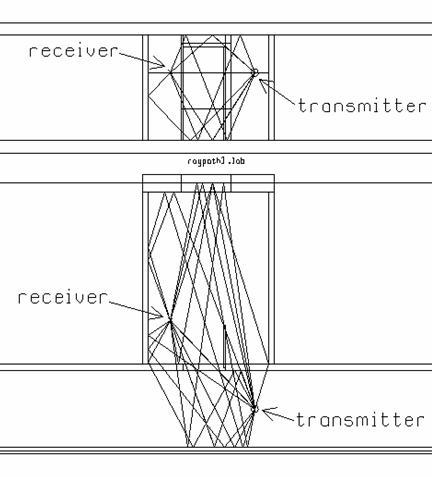
Figure 7(a) An observer with a line-of-sight path to the transmitter.
Fig.7(a) shows a receiver positioned in the room near the left-hand wall, such that there is a line-of-sight path to the transmitter. A modest threshold of 10 dB has been used to draw the ray paths. If a more sensitive threshold is used, the program will draw so many rays that the usefulness of the ray path drawing is lost. The drawing is useful in finding the principal rays connecting the transmitter to the receiver. Rays that are not transmitted through any wall often carry the largest field strength. Fig. 7(a) clearly shows a “direct” ray that travels from the transmitter, through the doorway, to the receiver. There are four more rays passing through the door. A ray travels from the transmitter, through the door, and then bounces from the room wall to arrive at the receiver. Another ray from the transmitter reflects from the hallway wall opposite the door, then travels through the doorway to the receiver. And there is a ray path that zig-zags, reflecting from the hallway wall near the door, then again from the hallway wall opposite the door, and then travels through the doorway to the receiver. The fourth ray travels from the source, reflects from the floor, and arrives at the receiver. Other rays are transmitted through a wall. There is a one-reflection path from the transmitter to the ceiling thence to the receiver but this ray passes through the transom above the door and so is attenuated by the transmission coefficient. Fig. 7 shows many ray paths that pass through the wall between the hallway and the room. Some of these rays bounce one or more times from the hall walls before passing into the room via transmission through the room walls. Some of the rays bounce from the room walls once or twice before reaching the transmitter. Quite a few rays bounce from the window glass, but this thin surface has a low reflection coefficient.
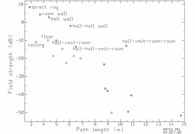
Fig. 7(b) The field strengths and path lengths for the rays at the line-of-sight observer.
Fig. 7(a) shows the field strengths, in dB re: 1 volt/meter, associated with the various rays arriving at the receiver, as a function of the ray path length. The circles show all the rays for a “three-dimensional” calculation, which includes the floor and the ceiling. To help in identifying ray paths, the same problem was run for a “two-dimensional” calculation by removing the floor and the ceiling from the problem, thus eliminating ray paths involving reflection from the floor or the ceiling. The “2D” ray paths are shown as crosses, so the circles without crosses are ray paths involving the ceiling or floor, or both. Specific ray paths can be identified with the aid of the “RAYLISTS” text file.
In Fig. 7(b), because there is a line-of-sight path to the transmitter, the largest field strength is associated with the ray having the shortest path length of 2.9 m, called the “direct” ray. The next longer path length is the reflection from the ceiling. The directional pattern of the dipole transmitter reduces the field of rays directed upward. This ray also passes through the wall above the doorway, with an associated transmission coefficient, and is attenuated by the ceiling reflection coefficient, so its field strength is 19 dB below the direct ray. The ray labeled “room wall” has the next longer path of 3.7 m has a single reflection from the room wall. The reflection from the floor has a path length of 4.3 m, but the field strength of this ray is small. The ray path labeled “hall wall” of path length of 4.4 m has a single reflection from the hall wall opposite the door and then passes through the doorway to the receiver. There is a ray labeled “hall-hall wall” in Fig. 7(b) that zigzags along the hall, with two reflections from the hall wall, then passes through the doorway to the receiver. A ray with a path length of about 5 m labeled “hall-xmit-room” reflects once from the hall wall, is transmitted through the room wall, and then reflects from the room side wall to reach the receiver. Due to the loss in transmission through the wall, the field strength associated with this ray is quite low. There is a ray labeled “hall-hall-xmit-room” which zig-zags along the hall, is transmitted through the hall wall into the room, and then reflects from the room wall to arrive at the receiver. Similarly, the “hall-xmit-room-room” ray reflects from the hall wall, is transmitted through the room wall into the room, then reflects twice from the room walls before reaching the receiver.
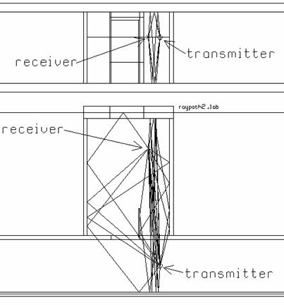
Fig. 8(a) A receiver which is not in the line-of-sight of the transmitter.
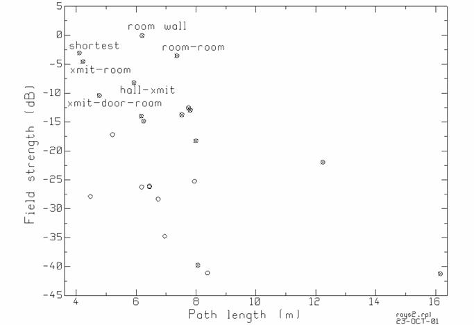
Fig. 8(b) The field strengths and path lengths for the rays of Fig. 8(a).
In contrast with Fig. 7(a), Fig. 8(a) shows a receiver that is not line-of-sight to the transmitter. There are still two coupling paths that pass through the doorway, but the delay times associated with these will be much longer than that of the shortest ray in Fig. 8(a). Fig. 8(b) shows the field strengths of the various rays as a function of the path lengths. The shortest path ray travels “directly” from the transmitted to the receiver with no reflections, but is transmitted through the hallway wall and so is reduced by the wall’s transmission coefficient. Thus, the field strength of the shortest-path ray is not the largest. The ray labeled “xmit-room” travels from the transmitter through the wall into the room and then reflects from the room wall before arriving at the receiver. The path length is only a little longer than the shortest ray and the ray is not greatly attenuated by the wall reflection, since incidence is near grazing. The ray labeled “xmit-door-room” is transmitted through the room wall, reflects from the door, reflects again from the room wall and arrives at the receiver. The double reflection further reduces the field strength. The point labeled “hall-xmit” is a ray that travels from the transmitter, reflects from the hall wall, travels through the room wall and into the room and arrives at the receiver. The field associated with this ray is reduced by the hall wall reflection coefficient for near-normal incidence and the transmission coefficient for the room wall. The rays with the strong field strengths are labeled “room wall” and “room-room”. The first travels through the doorway, reflects once from the wall and arrives at the receiver. The second travels through the doorway, and then zig-zags down the room with two wall reflections. It arrives at the receiver with a much longer delay time but with about the same field strength as the shortest ray. All of the ray paths in Fig. 8(a) could be identified from the “RAYLISTS” file, if needed.
5.2 Field Strength with Increasing Threshold
The “RCVRLINE” command of Table 1 can be used to ask the GO_3D
program to compute the field strength along a straight-line path between any
two points, such as the path from the center of the doorway to the window shown
as a dashed line in Fig. 5. The program
creates an output file giving ![]() ,
, ![]() ,
, ![]() and
and ![]() as a function of distance along the line. The horizontal axis can be chosen as distance
along the line, increasing from zero at the beginning of the line, or as
distance from the transmitter.
as a function of distance along the line. The horizontal axis can be chosen as distance
along the line, increasing from zero at the beginning of the line, or as
distance from the transmitter.
The threshold field strength T (dB) is a control that lets the user determine how sensitive a calculation is carried out by the GO_3D program. As explained above, GO_3D does not ask the user to set a limit on the number of reflections that the program will track. Instead, the code retains all image sources that could, for some observer, give rise to fields that are larger than the “cutoff” field strength, which is T dB below the isotropic level field strength. GO_3D will track as many reflections as needed to meet this criterion.
Table 2 shows the maximum number of reflections that the GO_3D code tracks for various threshold values for the hallway-with-room problem of Fig. 5. Also, the number of image sources that are needed is shown. With a 10 dB threshold, up to 7 reflections are tracked using a total of 426 image sources. With a 13 dB threshold, one more reflection is tracked and the number of image sources roughly doubles to 822. Note that the code does not find all the rays having 7 reflections, just those rays that might have field strength stronger than the threshold after 7 reflections. With a 16 dB threshold, up to 12 reflections are found using 1874 image sources. With a 19 dB threshold, 14 reflections are tracked using 7056 image sources. With a 22 dB threshold, 19 reflections are traced, using 26,037 image sources. With a 26 dB threshold the code tracks 29 reflections using 254,379 image sources. This very large numbers of image sources causes the code to execute quite slowly!
Table 2
The Number of Reflections and the Number of Image Sources for Various Threshold Values.
|
Threshold |
Reflections |
Image sources |
|
10 |
7 |
426 |
|
13 |
8 |
822 |
|
16 |
12 |
1874 |
|
19 |
14 |
7056 |
|
22 |
19 |
26037 |
|
26 |
29 |
254379 |
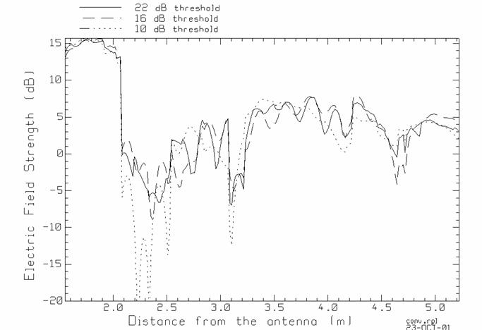
Figure 8 The field strength along the path in Figure 5, for various values of the threshold field strength.
Does the
field become constant as the value of the threshold increases? Ideally, we would like the field to
“converge” to a constant value as the threshold value is increased, and for
“large” thresholds, show little change for further threshold increase. But in general, this behavior is not found,
as illustrated in Figure 8. The figure
shows the field strength ![]() along the path in
Figure 5 from the center of the door into the room to the window, using
distance from the transmitter on the horizontal axis. The field is shown for thresholds of 10, 16,
and 22 dB. All four curves are similar
overall; they are dominated by a few rays that have relatively large field
strengths and are found by GO_3D even for the “low” 10 dB threshold value.
along the path in
Figure 5 from the center of the door into the room to the window, using
distance from the transmitter on the horizontal axis. The field is shown for thresholds of 10, 16,
and 22 dB. All four curves are similar
overall; they are dominated by a few rays that have relatively large field
strengths and are found by GO_3D even for the “low” 10 dB threshold value.
For close distances to the transmitter, there is a line-of-sight path from the transmitter to the observer and the behavior of the field is dominated by the large field strength of the “direct” ray from the transmitter. For all three threshold values the field for distances less than 2.07 m is very similar. By increasing the threshold value, the user instructs the code to include additional rays with fields at a much lower level than the “direct” ray’s field, which have only a small effect on the net field strength.
At 2.07 m distance the line of sight path is blocked by the wall, and for larger distances the field is made up of rays transmitted through the wall and reflected from various walls. With a 10 dB threshold only a modest number of rays contribute to the field, and there is a trough in the field strength from 2.07 m to 2.21 m distance. As the threshold is increased, a lot of “minor” rays are added which tend to fill in the trough, hence the field in this region with a 16 dB threshold is larger than with a 10 dB threshold. However, including even more “minor” rays by increasing the threshold to 22 dB does not increase the field in this trough further.
From about 2.6 to 3.1 m distance, and again from about 3.5 to about 4.2 m, the field with a “low” 10 dB threshold is fairly smooth. Increasing the threshold to 16 dB adds a ripple to the field called “fast” fading. The average value of the field, the “slow fading”, is not much changed. Increasing the threshold to 22 dB affects the amplitude of the ripple, but again the “slow fading” or average value is not much changed.
The results shown in this figure are typical of those obtained by increasing the threshold value in GO_3D. The field does not “converge” to a value independent of the threshold at all. Instead, adding more image sources by increasing the threshold fills in troughs found with low threshold values, and adds “fast fading” behavior to the overall curve.
Figure
9 The grid location is drawn on the
PLAN.LAB file.
5.3 Fields On a Planar Grid
The RCVRGRID command is used to ask the GO_3D program to report the
value of the ![]() ,
, ![]() ,
, ![]() and
and ![]() field strengths at a grid of points parallel
either to the xy, the xz or the yz plane.
For example, suppose a 600 mW transmitter is operated in the hallway,
and that the field in the rectangular region in the room in Fig. 9 must be
maintained less than, say, 3 V/m, to ensure electromagnetic compatibility with
equipment operated there. Then the
RCVRGRID command of Table 1 is used to fill the region with receivers, at a
spacing of 3.5 cm or about a tenth of the wavelength. When GO_3D is run, the field over the grid
can be graphed with CPLOT in the format shown in Fig. 10.
field strengths at a grid of points parallel
either to the xy, the xz or the yz plane.
For example, suppose a 600 mW transmitter is operated in the hallway,
and that the field in the rectangular region in the room in Fig. 9 must be
maintained less than, say, 3 V/m, to ensure electromagnetic compatibility with
equipment operated there. Then the
RCVRGRID command of Table 1 is used to fill the region with receivers, at a
spacing of 3.5 cm or about a tenth of the wavelength. When GO_3D is run, the field over the grid
can be graphed with CPLOT in the format shown in Fig. 10.
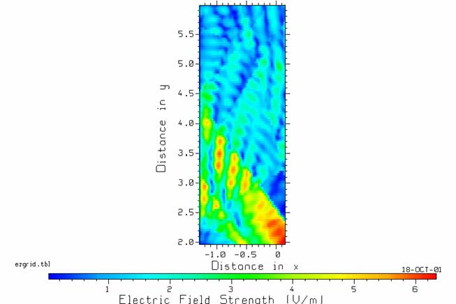
Figure 10 The ![]() component of the
electric field strength over the receiver grid.
component of the
electric field strength over the receiver grid.
Fig. 10 shows the ![]() component of the field
over the receiver grid of Fig. 9. This
“field map” was computed with a 18 dB threshold and a 3.5 cm point
spacing. The point at x=0,y=2 m near the
bottom right corner of the map is near the center of the doorway into the room,
and the field at this location is strong because it is “line of sight” to the
transmitter. All the points in the beam
flowing upward and to the left from the doorway in Fig. 10 are in the
line-of-sight. There is reflection of
rays from the wall at left, leading to a standing wave pattern at the center
left of the figure. The rays arriving at a typical observer in this region are
shown in Figure 7. Deeper in the room
there is no line-of-sight ray and the field is smaller in value, with colors
from blue to green. Some rays do arrive
at a typical receiver through the doorway, as shown in Figure 8. The room contains an interference pattern
showing maxima and minima which are oriented roughly vertically on the page,
and arise due to rays bouncing back and forth between the two walls of the
room.
component of the field
over the receiver grid of Fig. 9. This
“field map” was computed with a 18 dB threshold and a 3.5 cm point
spacing. The point at x=0,y=2 m near the
bottom right corner of the map is near the center of the doorway into the room,
and the field at this location is strong because it is “line of sight” to the
transmitter. All the points in the beam
flowing upward and to the left from the doorway in Fig. 10 are in the
line-of-sight. There is reflection of
rays from the wall at left, leading to a standing wave pattern at the center
left of the figure. The rays arriving at a typical observer in this region are
shown in Figure 7. Deeper in the room
there is no line-of-sight ray and the field is smaller in value, with colors
from blue to green. Some rays do arrive
at a typical receiver through the doorway, as shown in Figure 8. The room contains an interference pattern
showing maxima and minima which are oriented roughly vertically on the page,
and arise due to rays bouncing back and forth between the two walls of the
room.
6 Conclusions
GO_3D is a ray-tracing program for indoor propagation. The user prepares an input file giving the floor plan and the materials and construction of the walls. The transmitter location is specified, and the transmitter is modeled either as a half-wave dipole or as an “imported” source defined by a file of radiation patterns. The location of the observers or “receivers” is defined as either at one point, along a line or on a grid. The input “language” is intended to lead to a self-documenting file that is easy to read and modify. The user is encouraged to include comment lines in the file describing the contents, so that numbers in the file are readily traced to their source.
GO_3D computes the field strength either along a straight-line path defined by the user, or over a grid of points. The structure of the field in a region can be studied by drawing color contour maps of the field strength, as in Fig. 10. Using an observer at a single point, the GO_3D program creates output file that permit the study of the ray paths joining the transmitter to the receiver. Both the geometry of each ray, the length of the ray path and the field associated with it can be studied. Moving the observer in small steps permits the user to see which ray paths appear and disappear, and can help to explain features found in contour maps of the field over a region.
GO_3D provides a control called the “threshold” which allows the user to determine the number of rays to be included in the calculation. The value of threshold required for a given problem depends on the wall construction and on whether energy can escape from the problem region. Thus, if a closed room were built with perfectly-reflecting walls, then rays will continue to bounce around inside the room indefinitely with no decrease in field strength, and the ray tracing method breaks down. If the room has walls that permit some energy to escape through them, then the field amplitude associated with each ray gradually decreases with each reflection, but rays may have to be traced through many reflections to obtain an accurate answer. Such a room is very “live”. Conversely, a “dead” room is one that has many doorways and windows that allow rays to escape. Or it is a room with walls that permit energy to penetrate through them, or that absorb energy, and in either case have a small reflection coefficient. In such a “dead” room, only a few reflections need to be traced.
GO_3D uses geometrical optics and so ignore diffracted rays from edges such as the corners of walls and doorways. Consequently, the field has discontinuities as rays “switch” on and off with changing observer position. GO_3D does not model non-specular scattering, as might be expected from the clutter of conduits, plumbing and ducts found above a typical hanging ceiling. Nor does GO_3D permit the furnishing or contents of a room to be modeled. Perhaps some lossy “wall panels” could be included in a room to absorb some of the energy associated with the rays entering the room to approximate the effects of people and furniture.
The GO_3D program could be used as a teaching tool in undergraduate or graduate courses dealing with wireless technology and indoor propagation. Students could gain some first-hand experience by modeling a specific indoor environment, to become aware of the major considerations. The input for the program is quite simple to prepare, starting from the sample problem in the User’s Guide, and the program executes reasonably quickly on an inexpensive Pentium computer.
GO_3D has proven a useful tool for investigating the field in a room due to a transmitter located somewhere in the room, with reasonable correspondence to measurements[12]. The program has been used to study the decline in field strength with distance from the observer in long corridors[13]. The program has been used to study the locations in a corridor where a cellular telephone can be operated without exceeding the immunity level of equipment in an adjacent room[14], as in the example presented in this paper.
Acknowledgements
The author acknowledges the contribution of Dr. Junsheng Zhao in implementing the layered-wall reflection and transmission coefficients of Ref. [6], which have been borrowed from his geometrical optics code[ref paper submitted to Vehicular Technology]. The author acknowledges his colleagues Dr. B. Segal and D. Davis for inspiration in developing the GO_3D code to study EMC problems in a hospital environment.
References
1.
R.S. Rappaport, “Wireless
Communications, Principles and Practice”, Prentice Hall PTR,
2. R.K . Morrow, “Site-Specific Engineering for Indoor Wireless Communications”, Applied Microwave and Wireless, Vol. 11, No. 3, pp. 30-38, March ,1999.
3.
4. M. Kimpe, H. Leib, O. Maquelin, and T. D. Szymanski, “Fast Computational Techniques for Indoor Radio Channel Estimation”, Computing in Science & Engineering, pp. 31-41, Jan.-Feb., 1999.
5. C. Yang, B. Wu and C. Ko, “A Ray-Tracing Method for Modeling Indoor Wave Propagation and Penetration”, IEEE Trans. Antennas and Propagation, Vol. AP-46, No. 6, pp. 907-919, June 1998.
6.
E.H. Newman, “Plane Multilayer
Reflection Code”, Technical Report 712978-1, ElectroScience Laboratory, The
8. C.W. Trueman, program LABLNG.
9. C.W. Trueman, program RPLOT.
10. C.W. Trueman, program CPLOT.
11. J. Zhao, R. Paknys, and C.W. Trueman, “A Comparison of 2D and 3D Models for Indoor Propagation Prediction”, submitted for consideration for publication to the IEEE Trans. On Vehicular Technology.
12. C.W. Trueman, R. Paknys, J. Zhao, D. Davis, and B. Segal, “Ray Tracing Algorithm for Indoor Propagation,” ACES 16th Annual Review of Progress in Applied Computational Electromagnetics, pp. 493-500, Monterey, California, March 20-24, 2000.C.W. Trueman, D. Davis, and B. Segal, “Ray Optical Simulation of Indoor Corridor Propagation at 850 and 1900 MHz,” IEEE AP-S Conference on Antennas and Propagation for Wireless Communication, pp. 81-84, Waltham, Massachusetts, November 6-8, 2000.