User’s Guide for Program LAPL
September 15,
2000
Updated
C.W. Trueman
Introduction
Program LAPL solves
You can fetch a copy of the executable file for program LAPL by clicking this button: Get lapl.exe. You can fetch a copy of CPLOT by clicking this button: Get CPLOT.EXE. These programs run under Microsoft Windows.
Program LAPL solves ![]() . We want to find
. We want to find ![]() such that it satisfies
such that it satisfies
In two-dimensional problems, the
potential is a function of x and y only, so![]() . Then
. Then
![]()
We want to
solve a “boundary value” problem in which
Finite Difference Cell Space and Boundary Conditions
To solve ![]() m. The center of each cell is given by point
m. The center of each cell is given by point ![]() and the potential at
the center of the cell is given by
and the potential at
the center of the cell is given by ![]() . Note that LAPL views
the voltage
. Note that LAPL views
the voltage ![]() as being at the center of the cell, not at the left or
right side or at a corner of the cell. A
grid of
as being at the center of the cell, not at the left or
right side or at a corner of the cell. A
grid of![]() cells in the x direction by
cells in the x direction by ![]() cells in the y
direction permits us to represent cables with cross-sectional size as large as
cells in the y
direction permits us to represent cables with cross-sectional size as large as ![]() by
by ![]() m. The cells are numbered
m. The cells are numbered ![]() in the x direction
and
in the x direction
and ![]() in the y
direction.
in the y
direction.
Consider solving the metal trough
problem using the finite-difference method.
The trough measures ![]() m in the x direction
and b m in the y direction.
The bottom is the metal wall at y=0 and is grounded. The sides are the metal walls at x=0
and x=b and are also grounded.
The top is the metal wall at y=b and is assumed to be at 100
volts. Of course there must be an
insulator separating the upper end of the sides from the top, but the exact
size and geometry of the insulator are not usually specified in stating the
problem!
m in the x direction
and b m in the y direction.
The bottom is the metal wall at y=0 and is grounded. The sides are the metal walls at x=0
and x=b and are also grounded.
The top is the metal wall at y=b and is assumed to be at 100
volts. Of course there must be an
insulator separating the upper end of the sides from the top, but the exact
size and geometry of the insulator are not usually specified in stating the
problem!
To represent this problem for the
finite difference method we choose a cell size small enough to accurately
represent the spatial variation of the potential throughout the duct. Then choose the number of cells ![]() and
and ![]() by dividing the
dimensions of the duct by the cell size.
The potentials of all the cells on the edges of the cell space are fixed
in value using the boundary conditions. The
left-hand column of cells
by dividing the
dimensions of the duct by the cell size.
The potentials of all the cells on the edges of the cell space are fixed
in value using the boundary conditions. The
left-hand column of cells ![]() represent the
left-hand metal wall and have
represent the
left-hand metal wall and have ![]() =0. The right-hand
column of cells
=0. The right-hand
column of cells ![]() represent the right
wall and have
represent the right
wall and have ![]() =0. The bottom row of
cells
=0. The bottom row of
cells ![]() represent the bottom
metal wall of the trough and have
represent the bottom
metal wall of the trough and have ![]() =0. The top row of
cells
=0. The top row of
cells ![]() represent the top of
the trough which is at 100 volts, so for these cells
represent the top of
the trough which is at 100 volts, so for these cells ![]() =100 volts. All these cells all have fixed potentials and
are the “boundary conditions” for the problem.
To find the potential in the remaining cells, we have to solve
=100 volts. All these cells all have fixed potentials and
are the “boundary conditions” for the problem.
To find the potential in the remaining cells, we have to solve ![]() we want to solve
we want to solve ![]() .
.
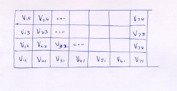
Fig. A Sketch of a 7 cell by 4 cell “cell space” with potentials numbered from the lower left corner.
Suppose we wish to model a 6 cm
wide by 3 cm tall duct with 1 cm cells.
The potential at the center of
cell #1,1 is ![]() . If we use 7 cells
across the duct, then the potential at the center
of cell #7,1 is
. If we use 7 cells
across the duct, then the potential at the center
of cell #7,1 is ![]() . The distance between
the center of cell #1,1 and the center of cell #7,1 is 6 cells or 6 cm,
correctly representing the width of the duct.
Similarly the height of the duct is represented with 4 cells so that the
distance from the center of cell #1,1
to the center of cell #1,4 is 3 cm. So a 6 x 3 cm duct is represented using 7
cells in the x direction and 4 cells in the y direction, as shown in Fig.
A.
. The distance between
the center of cell #1,1 and the center of cell #7,1 is 6 cells or 6 cm,
correctly representing the width of the duct.
Similarly the height of the duct is represented with 4 cells so that the
distance from the center of cell #1,1
to the center of cell #1,4 is 3 cm. So a 6 x 3 cm duct is represented using 7
cells in the x direction and 4 cells in the y direction, as shown in Fig.
A.
To enforce the boundary conditions,
set the edge cell potentials as follows.
On the left hand edge, the voltage is zero so set ![]() ,
, ![]() ,
, ![]() and
and ![]() . Across the bottom,
the voltage is zero so set
. Across the bottom,
the voltage is zero so set ![]() (done already),
(done already), ![]() ,
, ![]() , …, and
, …, and ![]() . On the right hand
edge, the voltage is zero so set
. On the right hand
edge, the voltage is zero so set ![]() (done already),
(done already), ![]() ,
, ![]() and
and ![]() . Across the top, we
consider
. Across the top, we
consider ![]() and
and ![]() to be part of the
sides of the duct. We want to set the
remaining five cells to the potential of the top of the duct, 100 volts, so set
to be part of the
sides of the duct. We want to set the
remaining five cells to the potential of the top of the duct, 100 volts, so set
![]() ,
, ![]() , …, and
, …, and ![]() . Then the potentials
inside the duct are
. Then the potentials
inside the duct are ![]() ,
, ![]() , …,
, …, ![]() , and
, and ![]() ,
, ![]() , …,
, …, ![]() , and these potentials must be found to satisfy
, and these potentials must be found to satisfy
Deriving the Update Equation
To use ![]() at the point half-wave
between
at the point half-wave
between ![]() and
and ![]() , we use
, we use
![]()
As an
exercise, write the formula that approximates ![]() at the point half-wave
between
at the point half-wave
between ![]() and
and ![]() . To approximate the
2nd derivative,
. To approximate the
2nd derivative, ![]() at point
at point ![]() , we use the approximation for
, we use the approximation for ![]() at the point half-wave
between
at the point half-wave
between ![]() and
and ![]() , minus the approximation for
, minus the approximation for ![]() at the point half-wave
between
at the point half-wave
between ![]() and
and ![]() . Hence
. Hence

With a
similar approximation for ![]() ,
,
![]()
This can be rearranged to obtain
![]()
In the finite-difference method, we rewrite this equation as
![]()
This is
called the “update equation, and is used to calculate a “new” value for ![]() from the values of the
potentials in the adjacent cells.
from the values of the
potentials in the adjacent cells.
The Finite-Difference Algorithm
The finite-difference algorithm
proceeds as follows. We start with an
“initial guess” for the potentials in the cells. This is usually zero potential: ![]() =0 for
=0 for ![]() . Then for
. Then for ![]() , and for
, and for ![]() use the “update
equation” to find a new value for each
use the “update
equation” to find a new value for each ![]() . This amounts to
replacing each voltage “inside” the trough with the average value of its four
neighbors. This is the first
iteration. Similarly, for the second
iteration, use the “update equation” to find a new value of
. This amounts to
replacing each voltage “inside” the trough with the average value of its four
neighbors. This is the first
iteration. Similarly, for the second
iteration, use the “update equation” to find a new value of ![]() for each point inside
the cell space,
for each point inside
the cell space, ![]() . Then do a third
iteration; then a fourth; and so on.
After a sufficient number of iterations, the potential values become
constant and we say that the solution has “converged” to its final value.
. Then do a third
iteration; then a fourth; and so on.
After a sufficient number of iterations, the potential values become
constant and we say that the solution has “converged” to its final value.
Returning to the problem of Fig. A,
we need to find ![]() ,
, ![]() , …,
, …, ![]() , and
, and ![]() ,
, ![]() , …,
, …, ![]() to satisfy the
difference equation
to satisfy the
difference equation
![]()
This is
done by iteration. Thus in the first
iteration, replace ![]() by the average value
of its four neighbors,
by the average value
of its four neighbors,
![]()
Then
replace ![]() by the average value
of its four neighbors, using the “new” value of
by the average value
of its four neighbors, using the “new” value of ![]() just calculated.
Replace
just calculated.
Replace ![]() by the average of its
four neighbors, replace
by the average of its
four neighbors, replace ![]() , then replace
, then replace ![]() . Then go on to the
next row. Replace
. Then go on to the
next row. Replace ![]() by the average value
of its four neighbors, then replace
by the average value
of its four neighbors, then replace ![]() by the average value
of its four neighbors, then replace
by the average value
of its four neighbors, then replace ![]() by the average of its
four neighbors, then replace
by the average of its
four neighbors, then replace ![]() , then replace
, then replace ![]() . This completes the
first “iteration”. The second iteration
is exactly the same: update
. This completes the
first “iteration”. The second iteration
is exactly the same: update ![]() , then
, then ![]() , then
, then ![]() then
then ![]() , then
, then ![]() . Then go on to the
next row, by updating
. Then go on to the
next row, by updating ![]() , then
, then ![]() , then
, then ![]() , then
, then ![]() , and finally
, and finally ![]() . This completes the
second iteration. After many iterations,
the values won’t change much from one iteration to the next and so we will know
that no further iterations are necessary.
. This completes the
second iteration. After many iterations,
the values won’t change much from one iteration to the next and so we will know
that no further iterations are necessary.
Program LAPL uses the
finite-difference method to solve
LAPL Input File Format
Table 1 lists the “commands” that program LAPL uses in its input file. Use your favorite text editor (the Notepad will work) or word processor to prepare a “txt” file describing your problem. Table 2 lists the file called “trough.txt” which describes a trough problem for solution with program LAPL.
The command “CM” permits you to include comments in the input file such as the name of the problem, the purpose of doing this problem, the date, and whatever other information that might help you to know what is in the file in a couple of years when you have forgotten all about what your were doing for this problem! In Table 2 the “CM” feature has been used to provide a brief description of each command, and also to identify the purpose of each “LINE” command defining the geometry.
The “SIZE” command defines the cell size in meters. Small cells resolve the geometry more precisely, especially in defining curved surfaces such as cylinders. But smaller cells lead to large cell space sizes, and then more computer time is needed for each iteration, and more iterations are needed overall for the solution to converge to a constant value.
The SPACE command defines the size of the cell space, 10 cells in x and 12 cells in y, which is very small. Usually much larger cell spaces are used.
The location of cells with fixed potentials must now be given, to define where the conductors are and what their potentials are. The LINE command is used to define either a horizontal row or a vertical column of cells at a fixed potential. In Table 1, the horizontal line of cells starting at cell 10,10 and ending at cell 20,10 is specified to be at 0 volts potential. Then the vertical line from cell 10,10 to cell 20,10 is specified to be at 100 volts. Lines must be horizontal or vertical. (This is bad and the program should be upgraded to handle diagonal lines!)
In Table 2, four line commands are
used as follows. The “bottom” of the
trough is set to zero volts. The left
and right side of the trough are set to zero volts. Then the top of the trough is set to 100
volts. This defines the potentials on the
four outer boundaries of the cell space.
However, by definition, the outer boundary of the cell space, namely the
bottom row, ![]() , the top row
, the top row![]() , the left-hand column
, the left-hand column![]() and the right-hand column
of cells
and the right-hand column
of cells![]() , must be at fixed potentials. The program assumes all of these cells are at
zero potential, unless the “LINE” command is used to change them. Thus in Table 2, the LINE commands fixing
three of the boundaries to zero potential are not really necessary and could be
omitted.
, must be at fixed potentials. The program assumes all of these cells are at
zero potential, unless the “LINE” command is used to change them. Thus in Table 2, the LINE commands fixing
three of the boundaries to zero potential are not really necessary and could be
omitted.
Three more commands let the user specify input geometry. Infinitely-long cylindrical wires are frequently used in two-dimensional problems. These have a circular cross-section and are described with the “CIRCLE” command. “CIRCLE” specifies the cell at the center of the wire (cell 50,50 in Table 1), the radius of the wire in cells (10 cells in Table 1), and the potential of the wire. Hollow cylinders such as the outer conductor of coaxial cable are also frequently used. “CSHELL” or “Cylindrical Shell” is used to specify a hollow cylinder, having its center at cell 50,50 in Table 1, and a radius of 40 cells. The shell is 1 cell thick, by definition. “ELLIPSE” is used to describe an elliptical, hollow shell. In Table 1, the ellipse has its center at cell 50,50. The horizontal axis of the ellipse has a half-length of 60 cells and the vertical axis has a half-length of 30 cells. This can be used to model the outer conductor of a “coaxial” cable of radius 50 cells that has been squashed or distorted into an ellipse having a horizontal “radius” of 60 cells and a vertical “radius” of 30 cells.
The finite-difference method must approximate curved surfaces such as cylinders with a “staircase” of rectangular cells. This has a profound effect on the accuracy of the results that can be obtained by this method, and is discussed further in the example on coaxial cable, below.
Program Control Commands
The next group of commands in Table 1 let the user control the execution of the finite-difference method. The total number of iterations that the program will perform is specified with NSTOP and is usually much larger than 10. For large cell spaces of 100 by 100 or more, values of NSTOP of 10,000 or even larger are often needed.
Note that program LAPL does not include any method for “automatically” terminating execution when the voltages have “converged” to sufficiently constant values. Thus, some finite-difference codes examine the change in the potentials from one iteration to the next. If the change is less than a pre-set amount, such as one percent of the largest fixed potential, then the program would terminate automatically. In LAPL the user must guess the number of iterations required for convergence and specify it with NSTOP. Watch the screen to see if the potentials have become constant as iterations are done at the end of your “run” of LAPL.
If SINGLESTEP is included in the input file, the program updates one cell, draws the color of the updated cell to the screen, then pauses and waits for the user to press “return”. This is handy for demonstrating the update process for very small cell spaces, such as the 10 by 12 space in Table 2. For most purposes SINGLESTEP is not included in the input file.
As the program executes it draws the potential distribution to the screen. Drawing slows down execution. The user can specify the number of iterations to be performed before updating the potential distribution on the screen. Use the NUPDATE command. In Table 1, NUPDATE is used to ask that the screen be updated after 10 iterations have been done; updates after 100 or 1000 iterations are more commonly used.
LAPL normally updates the screen and then continues on with the calculation. If you want the program to pause after updating the potentials, then include PAUSE in your input file. The program waits while you examine the screen. Push “return” and the program will continue doing iterations. Use PAUSE with small cell spaces. With large cell spaces, performing iterations is sufficiently slow (at least on my 266 MHz laptop) that you have plenty of time to examine the potentials before the next update of the screen.
Capacitance per Unit Length
To calculate the
capacitance-per-unit-length of a structure such as coaxial cable, we need to
know the charge-per-unit-length on the inner conductor, ![]() C/m. Then the capacitance-per-unit-length is
C/m. Then the capacitance-per-unit-length is
![]() F/m
F/m
where V is the potential that we have specified on the inner conductor relative to the outer conductor. The charge-per-unit-length can be found using Gauss’ Law. Thus we need to specify a closed surface that encloses the center conductor. In program LAPL we can use the GAUSS command to define a rectangular box in the cell space. In Table 1, the corners of this box are cell 10,20 at the lower left and cell 80,90 at the upper right. The Gaussian box must lie entirely within the dielectric region of the problem, with the center conductor entirely inside the box. Program LAPL evaluates the charge-per-unit-length in each cell inside the Gaussian box and sums up all the charges to find the net charge-per-unit-length inside the box. Of course, the charge in the free-space cells is zero, and the charge inside conductors is zero. The charge resides on the surfaces of the conductors. When GAUSS is used, the program reports the charge inside the Gaussian surface to the screen before the program terminates execution.
The “END” Command
The “END” command is used to mark the end of the input file. Program “LAPL” does not do anything with the “END” command. But it is useful to include END so that you know that you have the complete input file, and nothing is missing.
Running the LAPL Program
Run the program by typing “LAPL” in a DOS window or double-clicking on file name LAPL.EXE in a directory window. Type the name of the input file into the box on the screen. Then push F10 and execution will begin. The program draws the cell space, showing grounded cells as black, and cells with a specified potential in the appropriate color using the color scale at the bottom of the screen. The program pauses to permit the user to look at the geometry and examine it for errors. Push “return” to start the calculations.
When the program is running, the user can push the “s” key (meaning for “stop”) to terminate the execution. After each iteration the program checks the keyboard to determine if “s” has been pressed and if so the program exits without writing any output files, and the results of the calculation are lost.
If SINGLESTEP has been included in the input file, push return to go on to updating the next cell. This is used to demonstrate the updating equation cell by cell for small cell spaces. SINGLESTEP is not included for “large” cell spaces!
During execution, LAPL performs the number of iterations specified with the NUPDATE command and then redraws the potentials to the screen. If the PAUSE command has been included in the input file, then the program waits while the user examines the screen and then presses “return” to continue. If PAUSE was not included the program carries on execution and then updates the screen after the specified number of iterations.
After the total number of iterations specified with NSTOP have been completed, the program displays the final values of the potentials and waits for the user to push “return”. If a Gaussian surface has been defined with the GAUSS command, the program reports the charge per unit length to the screen. Then the program writes the output files VOLTS.TBL and EFIELD.TBL, and terminates. Use program CPLOT to display the contents of the two TBL files.
The following sections solve some simple problems with program LAPL.
Table 1
Input Commands for Program LAPL
|
Purpose |
Command |
|
Include a descriptive comment in the input file |
CM followed by your text |
|
Specify the cell size (meters) |
SIZE 0.01 |
|
Specify the size of the finite-difference cell space |
SPACE 10 12 |
|
Define a line of cells at a fixed potential |
LINE 10 10 20 10 0. LINE 10 10 10 20 100. |
|
Define a solid cylinder of cells at a fixed potential |
CIRCLE 50 50 10 100. |
|
Define a hollow cylindrical shell of cells at a fixed potential |
CSHELL 50 50 40 0. |
|
Define a hollow elliptical shell of cells at a fixed potential |
ELLIPSE 50 50 60 30 0. |
|
Specify the total number of iterations to be done |
NSTOP 10 |
|
Pause the program after updating each cell |
SINGLESTEP |
|
Redraw the potentials after 10 iterations of updating the cell space |
NUPDATE 10 |
|
Pause the program after redrawing the potentials |
PAUSE |
|
Define a Gaussian Surface |
GAUSS 10 20 80 90 |
|
Mark the end of the input file |
END |
Table 2
The input file “trough.txt”
for a rectangular trough problem.
|
CM
Rectangular metallic trough with grounded bottom and sides CM
and with the top at 100 volts. CM CM
Size of the cells in meters: SIZE 0.01 CM CM
Size of the finite-difference cell space: SPACE
12 10 CM CM
Define the walls of the trough, and their potentials: CM
bottom: LINE 1
1 12 1
0. CM
left side: LINE 1
1 1 10
0. CM
right side: LINE 12
1 12 10
0. CM
top at 100 volts: LINE 1
10 12 10
100. CM
Total number of iterations to be done: NSTOP 10 CM CM
Pause the program after updating each individual cell: SINGLESTEP CM CM
Mark the end of the file: END |
Demonstrating the Update Equation
The input file of Table 1 can be used to demonstrate the results of applying the update equation to a problem cell by cell. Run LAPL and type the name of the input file. Then push F10 to get the display in Fig. 1, which shows the cell space defined in Table 1, of size 10 by 12 cells. The bottom and two sides are grounded cells, shown in black, and the top is set to 100 volts. The color scale at bottom displays the voltages using a range of colors from white for zero or small potentials, through blue, cyan, green, yellow, orange and red for cells at or near 100 volts potential. Push “return” to start the finite-difference calculation.
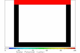
Figure 1 The “small trough” problem.
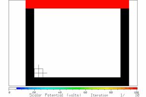
Figure 2 The cell space after updating the first cell.
Figure 2 shows the cell space after applying the update equation to the first cell. The result is zero potential because the four surrounding cells all have zero potential. Keep pressing “return” until the cell at the upper left corner is updated; it is the first that has a non-zero neighbor and so is assigned a non-zero value, as in Figure 3. Note that the LAPL program steps through the cell space by columns, not by rows.
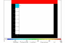
Figure 3 The results of updating the first column of cells.
Hold down the return key until all the cells inside the cell space have been updated, as in Figure 4, and the first iteration is complete. The only non-zero cells are those adjacent to the top of the cell space.
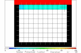
Figure 4 The potentials after one iteration.
Keep pressing “return” until the second iteration is complete to obtain the display in Figure 5. After two iterations, the two rows of “variable” cells at the top have non-zero values. The cyan cells of Figure 4 have increased in potential to become green cells, and the next row of cells have been assigned potentials of about 10 volts represented with a dark blue color.
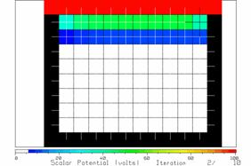
Figure 5 The potentials after two iterations.
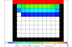
Figure 6 The potentials after four iterations.
Keep holding down the “return” key and watch the potentials change. After 4 iterations, there are three rows of non-zero potentials as shown in Fig. 6. At each iteration the non-zero potentials move down further in the trough. After 10 iterations, the potentials are still near zero in the bottom three rows of interior cells and the solution has not “converged” to constant values as yet.
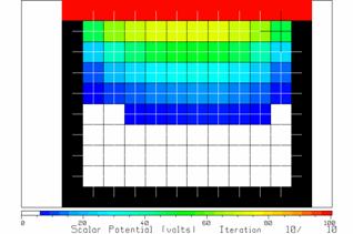
Figure 7 The potentials after 10 iterations.
It is tedious to watch the program update the potentials cell-by-cell. Hence, remove SINGLESTEP from the input file. Change NSTOP to 100, and add NUPDATE 10 so that the program will update the screen after doing 10 iterations, and PAUSE so that the program will wait after each screen update so that we can examine the potential distribution. This lets us look for convergence in jumps of 10 iterations.
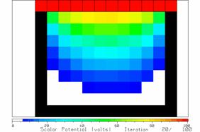
Figure 8 The potentials after 20 iterations.

Figure 9 The potentials after 50 iterations.
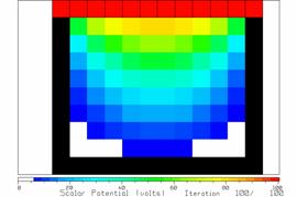
Figure 10 The potentials after 100 iterations.
Figure 8 shows the potentials after 20 iterations, quite different from those after 10 iterations. After 30 and 40 iterations, enough changes in the potentials are seen to warrant further iteration. But after 50 iterations, little change is seen. Compare Figure 9 after 50 iterations with Figure 10 after 100 iterations. There is little change in the solution.
Coaxial Cable
As a second example of the operation of the update equation, consider solving for the potentials in a coaxial cable. Figure 11 shows a coaxial cable using a “crude” cell space of 20 by 20 cells. The inner conductor radius is 10 cells. The red region in Fig. 11 is a “staircased” approximation to a round inner conductor. This is a crude approximation of a smooth cylindrical surface in terms of square cells. We expect that the electric field will be largest at the sharp corners of the cells. The outer conductor is approximated by a “staircase” of cells with a radius of 10 cells, and is also a crude approximation of a circle.
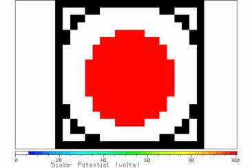
Figure 11 A model of a coaxial cable.
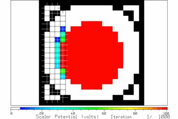
Figure 12 The potentials after four columns of cells at left have been updated.
In the single step mode, the results of updating each cell can be seen. Fig. 12 shows the potentials after updating four columns of cells. Some cells adjacent to the center conductor acquire non-zero values.
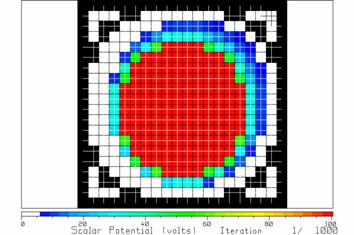
Fig. 13 The potentials after one iteration.
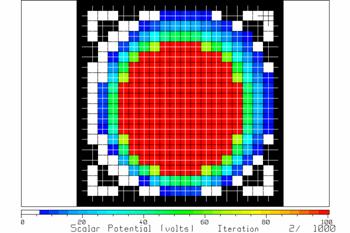
Fig. 14 The potentials after two iterations.
After two iterations, the potentials are as in Fig. 14. It does not take many iterations to reach steady state in this problem. Fig. 15 shows the potentials after 10 iterations.
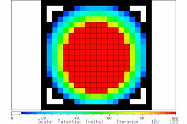
Fig. 15 The potentials change little from one iteration to the next after 10 iterations.
Trough Using a Larger Cell Space
The precision of the potential distribution using 10 by 12 cells is quite poor. Geometrical features are resolved to about a half a cell size. To get a finer resolution of the geometry we must use much smaller cells, but then we must do much more iteration to find the solution.
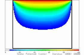
Figure 16 A 100 by 120 cell model of the trough, showing the
potentials after 1000 iterations.
Fig. 16 shows a 100 by 120 cell representation of the trough problem, using 10 cells for every cell in the previous problem. This resolves geometrical distances 10 times more finely than before. Start LAPL and type your file name for this problem, then push F10 to see the geometry. Push “return” to start the iteration. Now you must be patient because 1000 iterations with this large cell space takes a bit of time. Fig. 11 shows the potentials after 1000 iterations. The non-zero potentials have not propagated all the way to the bottom and more iterations are necessary.
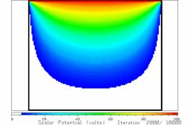
Figure 17 The potentials after 2000 iterations.
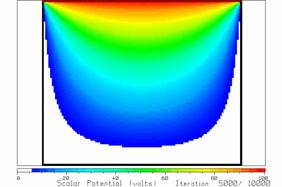
Figure 18 The potentials after 5000 iterations.
Figures 17 and 18 show the potentials after 2000 and 5000 iterations, respectively. There is significant change from 2000 to 3000 to 4000 to 5000 iterations. By 7000 iterations it is hard to see and change in the potentials and the solution has “converged”. Fig. 19 shows the potential after 10,000 iterations. Note that when we make the cell size 10 times smaller, it takes about 102=100 times as many iterations to “converge” and each iteration takes about 100 times longer to carry out. So increased precision in resolving the geometry comes at a steep cost in increased computer time.
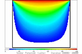
Figure 19 The potentials after 10,000 iterations.
Modeling Coaxial Cable
Coaxial cable consists of a metal inner conductor of radius a surrounded by hollow cylindrical metal outer conductor of inner radius b. Given values for the radii, say a= 1mm and b=5 mm, the finite-difference method can be used to find the capacitance per unit length of the cable, and the maximum electric field in the cable. Since we know the “theoretical” solution, we can compare the approximate values obtained from a finite-difference solution with the exact values.
Consider a coaxial cable
with air dielectric, a center conductor of diameter 2a=1 mm and an outer
conductor of inside diameter 2b=5 mm.
We are asked to find: (1) the maximum voltage that the cable can sustain
if the dielectric strength of the air is 3 megavolts/meter; and (2) the
capacitance-per-unit-length.
To model the cable, we will
choose the cell size such that the outer conductor is 100 cells in diameter,
hence
![]() meters.
meters.
Then the inner conductor is of diameter 20 cells. Table 3 lists the input file. The SPACE size is 100 by 100 cells. The CELL size is 0.00005 meters. The cross-section of the inner conductor is
represented as a circle centered at cell 50,50, with radius 10 cells, and at a
potential of 100 volts. The outer
conductor is represented as a hollow cylindrical shell centered at cell 50,50,
with radius 50 cells, at a potential of zero volts. Figure 20 shows the geometry. The square cell space has grounded cells all
the way around its outer boundary, by default.
Inside the square outer boundary the CSHELL command inscribes a circle
of cells of diameter 100 cells, all grounded.
We “waste” the cells in each corner of the square. They are outside the coaxial cable and the
potentials in these cells are of no interest.
In fact since these four “triangular” regions are surrounded by grounded
cells, the potentials will always be zero inside.
Table 3 specifies that the
program carry out 1000 iterations. The
screen is updated after every 100 iterations.
We must inspect the potentials to see that there is little change from
iteration 800 to 900 to 1000, to be sure the solution has converged to constant
values. The PAUSE command is included so
that the program will wait while we inspect the screen.
Since we are trying to calculate
the capacitance-per-unit-length, we need to know the charge-per-unit-length
that resides on the inner conductor when it is at 100 volts. Hence a GAUSSian surface has been defined
with corners at cell 20,20 and at cell 80,80.
In Figure 20 the Gaussian surface is drawn as a square surrounding the
inner conductor.
Table 3
Input file for the coaxial
cable problem.
|
CM
Coaxial Cable Problem CM CM
Inner conductor 1 mm diameter = 10 cells CM
Outer conductor 100 cells diameter. CM SPACE
100 100 CM CM
CELLSIZE (in meters) SIZE 0.00005 CM CM
Inner conductor: CIRCLE 50
50 10 100. CM
Outer Conductor: CSHELL 50
50 50 0. CM CM
Total number of iterations: NSTOP 1000 CM
Number of iterations before redrawing the graphics screen: NUPDATE 100 CM
Pause the display after each screen update: PAUSE CM
Gaussian Surface for evaluating the charge inside: GAUSS 20 20
80 80 CM CM END |
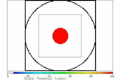
Figure 20 The geometry for
the coaxial cable problem.
Fig. 20 shows that the smooth round curves of the cylinders are approximated as a jagged edge of square cells. As previously mentioned, this is called a “staircased” approximation. In general the fields associated with a staircased surface are similar to those of the actual smooth surface if the observer is more than a couple of cells away from the surface. But the field within one cell of the staircased surface may not be a good approximation to the field of the true, smooth surface. In particular, the electric field is smaller than expected where the staircase is very flat, for example at the left edge and right edge of the center conductor. Conversely, the field is largest around the sharp corners of the cells where the staircase represents a diagonal line. In the following the results computed with the finite-difference method will be compared to those of the exact solution for the coaxial cable, to assess the error that staircasing incurs.
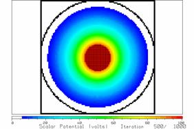
Fig. 21 After 500 iterations.
Fig. 22 After 800 iterations.
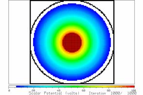
Fig. 23 After 1000 iterations.
With the input file in Table
3, program LAPL can be run. After 500
iterations, the solution is that in Fig. 21.
After 800 iterations it is somewhat different, as in Fig. 22, and after
1000 iterations, Fig. 23. But between
800 and 1000 iterations there is little change so we conclude that 1000
iterations is sufficient for the solution to “converge”. Note that in these drawings, the cells
representing the center conductor, whose potential is fixed at 100 volts, are
outlined in black. This distinguishes
them from the cells surrounding the center conductor, which are also at
potentials near 100 volts. Fig. 23 shows
what we would expect for the scalar potential or voltage distribution inside a
coaxial cable. That is, the
equipotentials are circles surrounding the center conductor. The strongest potentials are found at the
center conductor’s surface, decreasing rapidly then more slowly towards the
outer conductor.
Before LAPL terminates, it reports that the charge-per-unit-length inside the Gaussian surface is 3.55 nC/m. Before the program finishes it writes two files, VOLTS.TBL and EFIELD.TBL. In the following, program CPLOT will be used to examine the potentials and fields found in these files.
Using CPLOT to Draw the Scalar Potential Distribution
The files that LAPL creates with extension TBL are intended to be displayed with the color contour-mapping program called “CPLOT.exe”. To display VOLTS.TBL, run CPLOT and type the file name, then F10. This gets CPLOT’s main menu. Press F3 to get a color map of the potential distribution as a function of x and y as shown in Fig. 24. Note that the “tbl” file contains the character strings for the axis labels and the title of the color scale at the bottom. It is sometimes useful to reset CPLOT’s transformation from voltages into colors to be linear, by typing F4 then F1, then F10 to return to CPLOT’s main menu.
CPLOT’s display of Fig. 24 is very similar to Fig. 23, drawn by program LAPL itself. CPLOT does not “know” where the fixed potential or grounded cells are located, however, so cannot include these in the drawing. Also CPLOT does not use white to represent zero volts. Instead CPLOT uses the darkest blue color. Another subtle difference is that in LAPL the voltage is constant over each cell, but in CPLOT the voltage is graphed as varying linearly from one cell center to the next.

Fig. 24 CPLOT’s display of the voltage distribution in VOLTS.TBL.
The plotting mode in CPLOT is “color map with black contour lines”, and so we see lines of equal potential at 0, 20, 40, 60, 80 and 100 volts in Fig. 24. We can add labels to these contours by typing F7 then F1. Use the mouse to point to each contour in turn and then click the right mouse button; this generates a label for the contour. Click the left mouse button to finish, then F10 to return to the main menu and F3 to plot. Fig. 25 shows the potential distribution with labeled contour lines.
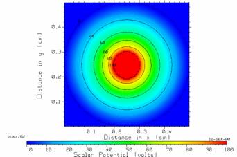
Fig. 25 CPLOT’s display of contours of constant potential.
In Fig. 25 note that the contours for 20, 40, 60 and 80 volts are quite circular, which is exactly what is expected from the theoretical solution for coaxial cable. However, the contours for 0 volts and 100 volts are jagged. These contours reflect the underlying staircased approximation to the true potential function.
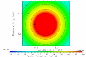
Fig. 26 Enlargement of the center portion of the scalar potential graph of Fig. 20.
CPLOT permits enlarging any part of the contour map to fill the screen, called “zooming”. Type F2 then F2 again; use the left mouse button to drag the edges of the “zoom box” to enclose the center conductor and press the right mouse to exit. Fig.26 shows the resulting display. We see that the 100 volt contour is jagged, showing the corners of the finite-difference cells clearly. The potential near the surface of the center conductor is about 100 volts everywhere.
Graphing the Magnitude of
the Electric Field
Once the scalar potential distribution ![]() has been found, then
the electric field can be evaluated using
has been found, then
the electric field can be evaluated using
![]()
Using the finite-difference approximation, the scalar potential is
known only at the centers of the cells, ![]() . The
central-difference formula is used to approximate the partial derivatives. Hence the electric field vector is computed
as
. The
central-difference formula is used to approximate the partial derivatives. Hence the electric field vector is computed
as
![]()
and the magnitude of the electric is found as
![]()
Program LAPL evaluates the magnitude of the electric field throughout the cell space and writes the field values to a file called EFIELD.TBL for graphing with CPLOT. Note that the file contains only the magnitude of the electric field and not its vector components.
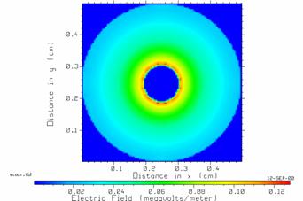
Fig. 27 The magnitude of the electric field in the coaxial cable.
For the coaxial cable problem CPLOT can be used to obtain the electric field distribution of Fig. 27. As expected the electric field is large near the surface of the center conductor and much smaller towards the outer conductor. Fig. 28 is an enlargement of the center of Fig. 27.
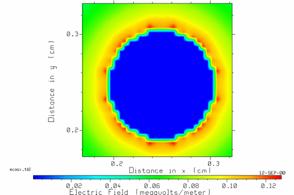
Fig. 28 The electric field magnitude surrounding the center conductor.
Fig. 28 requires some thought to interpret. The red spots are the regions of high electric field. As expected, they occur at the corners of the cells “staircasing” the curved surface of the center conductor. The field inside the center conductor should be zero everywhere, graphed as a region of dark blue. CPLOT uses a linear increase in field magnitude from the zero-field cells inside the center conductor to the high field points just outside the surface, hence the color starts as blue in the center conductor then passes through cyan, green and yellow to reach red at some points near the surface. This is not a realistic interpretation; the field strength should abruptly jump from zero just below the surface of the center conductor to a large value just outside the surface. But CPLOT is a general-purpose contour mapping program and does not “know” this. CPLOT does the best it can with the linear interpolation approach and we must interpret the resulting graph knowledgably.
To find the largest field strength in the cable using CPLOT, type F5 to obtain the scale menu. The “largest Z-value” is reported as 0.1279 megavolts/meter and is the largest electric field magnitude found inside the cable.
In a coaxial cable with a smoothly curved cylindrical center conductor, the electric field magnitude is given by
![]()
where r is the radial distance from the center of the
cable. The field is largest all around
the center conductor at r=a. The finite-difference approximation of Fig.
28 is quite different. The electric
field magnitude is large at the corners of the cells approximating the shape of
the center conductor, instead of being uniformly large all around the center
conductor. Hence, we might not expect
the largest electric field strength in the finite-difference approximation of
the coaxial cable to be in good agreement with the theoretical maximum value of
![]() V/m. For dimensions of 2a=1 mm and 2b=5
mm, and V=100 volts, we find
V/m. For dimensions of 2a=1 mm and 2b=5
mm, and V=100 volts, we find
![]() 0.1243 megavolts/meter
0.1243 megavolts/meter
Compare this with the finite-difference value of 0.1279 megavolts/meter. The finite-difference method’s error is about 3 percent. This is much more accurate that might be expected, considering that the “staircased” approximation to the center conductor is so crude compared to a true cylinder.
The Maximum Voltage that
the Cable Can Sustain
With 100 volts between the center and the outer conductor, the field in the cable is 0.1243 megavolts/meter. How much voltage is required for the field to be equal to the breakdown strength of air, 3 megavolts/meter? Since the largest field strength varies linearly with the voltage, simply multiply the voltage by 3/0.1243, hence
![]() volts
volts
is the largest voltage that the cable can sustain without breakdown of the air dielectric. The value for the maximum electric field magnitude using the finite-difference approximation is 0.1279 megavolts/meter, leading to a maximum voltage of 2346 volts. This underestimates the voltage that the cable can sustain by about 3 percent, since the largest field was overestimated by about 3 percent. The estimate is conservative, in the sense that the cable can actually sustain a larger voltage than we are expecting that it will.
Capacitance-Per-Unit-Length
The theoretical formula for the capacitance-per-unit-length of coaxial cable is
![]() 34.57 pF/m
34.57 pF/m
This is the exact value. To estimate the capacitance-per-unit-length, use the formula
![]() F/m
F/m
where ![]() is the
charge-per-unit-length on the center conductor corresponding to a voltage of V
volts. In the input file in Table 3, a
GAUSS command has been used to define a Gaussian surface that encloses the
center conductor, shown in Fig. 20. When
LAPL is run, it reports that the charge-per-unit-length inside the Gaussian
surface is 3.55 nC/m corresponding to a voltage of 100 volts on the center
conductor. Hence the
capacitance-per-unit-length is estimated as
is the
charge-per-unit-length on the center conductor corresponding to a voltage of V
volts. In the input file in Table 3, a
GAUSS command has been used to define a Gaussian surface that encloses the
center conductor, shown in Fig. 20. When
LAPL is run, it reports that the charge-per-unit-length inside the Gaussian
surface is 3.55 nC/m corresponding to a voltage of 100 volts on the center
conductor. Hence the
capacitance-per-unit-length is estimated as
![]() pF/m
pF/m
This is an error of about three percent compared to the exact value.
A “TEM Cell”
A two-conductor transmission line is sometimes made with a large outer conductor of rectangular cross-section, surrounding a flat, rectangular center conductor, as shown in Fig. 29. This arrangement is called a “TEM cell” and is used to obtain a region of space where the electric field strength is very uniform and has a well-known value. Then equipment can be place inside the TEM cell to determine if it can operate correctly when exposed to the cell’s electric field.
As an example of TEM cell geometry, use an outer conductor of width 100 cm and the height 50 cm. The center conductor, often called the “septum”, is 80 cm wide by 2 cm tall, and is centered in the outer box. The problem is to find: (1) the value of the electric field in the uniform region of the TEM cell, with 100 volts on the septum; (2) the largest electric field; and (3) the capacitance-per-unit-length.
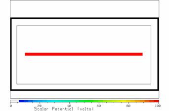
Fig. 29 A rectangular, grounded metal box surrounding a septum at 100 volts.
To model this transmission line, use a cell size of 1 cm, so that the cell space is 100 by 50 cells and the septum is 80 by 2 cells. Fig. 29 shows the geometry. The outer wall uses grounded (black) cells. The septum uses cells at 100 volts(red). The light rectangle is the Gaussian surface to be used to find the charge-per-unit-length on the center conductor.
Program LAPL is run for 1000 iterations. After 500 iterations, the scalar potential changes little with further iteration. LAPL reports the charge inside the Gaussian surface is 8.278 nC/m. Fig. 30 shows the scalar potential after 1000 iterations. The voltage between the central region of the septum and the bottom (or top) wall is very uniform and very like that in a parallel-plate capacitor.
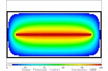
Fig. 30 The scalar potential after 1000 iterations.
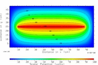
Fig. 31 The scalar potential in the TEM cell, drawn with CPLOT.
CPLOT can be used to draw equipotentials lines, using the VOLTS.TBL file. In the central region between the septum and the bottom of the box, the equipotentials lines are nearly parallel, and are evenly spaced between the septum and the bottom wall. This suggests that the electric field is very uniform.
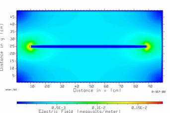
Figure 32 The electric field magnitude in the TEM cell.
Graphing the file EFIELD.TBL with CPLOT obtains the contour map of the magnitude of the electric field of Fig. 32. As is expected the largest electric field value occurs at the corners of the septum. CPLOT reports that the largest field strength is 0.001807 megavolts/meter or 1.807 kilovolts/meter. To find the field in the uniform region, position the cursor in this region with the mouse and click the left mouse button. The field is reported as 0.419 kilovolts/meter.
The capacitance per unit length is found from LAPL’s value for the charge inside the Gaussian surface, corresponding to 100 volts on the inner conductor, of 8.28 nC/m. This obtains
![]() pF/m
pF/m
This is the estimate of the capacitance per unit length of the TEM cell “transmission line”.
Some Hints for Using CPLOT
This section contains some hints for using CPLOT effectively for graphing the potential distribution VOLTS.TBL and the electric field magnitude EFIELD.TBL.
CPLOT graphs ![]() where z is the
value of the function at each point x,y on the screen. The x axis runs horizontally and the y
axis vertically. The z data can graphed
either on a linear scale or in decibels.
For the dB scale the data must all be positive, with no zero
values. Typing F5 gets the scale
menu. On this menu you can enter a title
for the z axis, which appears under the spectrum bar at the bottom of
the screen.
where z is the
value of the function at each point x,y on the screen. The x axis runs horizontally and the y
axis vertically. The z data can graphed
either on a linear scale or in decibels.
For the dB scale the data must all be positive, with no zero
values. Typing F5 gets the scale
menu. On this menu you can enter a title
for the z axis, which appears under the spectrum bar at the bottom of
the screen.
CPLOT has five modes of operation. Select a mode with F9. The modes are: (1) color map only; (2) color map with white contour lines; (3) color map with black contour lines; (4) contour lines drawn in color on a white background; and (5) black contour lines on a white background. This last mode creates a traditional line-drawing contour map, useful for preparing reports that must be printed in black ink on white paper, with no color.
The key to an effective color contour map is the conversion of z values to colors. CPLOT provides controls for this conversion in the F5 “axis format” menu and in the F4 “color scale” menu. The F5 menu gives control of the color scale as follows. The color spectrum bar runs from “ZLOW” to “ZHIGH”. Data values from ZLOW to ZBLACK are plotted in black. Field values from ZBLACK to ZWHITE are plotted in color (from blue to red), and data values from ZWHITE to ZHIGH are plotted in white. For most purposes choose ZLOW=ZBLACK and ZWHITE=ZHIGH. Also, very often ZLOW is set equal to the smallest value in the z data and ZHIGH to the largest z value, but in some applications a more appropriate choice can be made.
In the range from ZBLACK to ZWHITE, the program must map z values into colors. This is controlled with the “color scale” menu or F4 menu. The transformation from z values to colors is defined in terms of three straight-line segments. Use F1 in the color scale menu to reset the transformation to a simple straight line, then type F3 to see the transformation on the screen, as shown in Fig. 33.
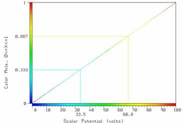
Fig. 33 The transformation from z values to colors.
The color scale menu gives you control of two “break points”. By typing F1, these are set to give a linear relation between the voltage and the color, as shown in Fig. 33. Thus the break points are set at a voltage of 33.5 and a color value of 0.333, and a voltage of 66.8 and color value of 0.667. You can raise or lower any of these four values to map z values into colors in a different way. This can be useful if you want to emphasize a small range of z values by using a lot of colors to graph them, for example.
It can be handy to completely reset the color scale. Type F5 then F6 then F5. This resets to a linear scale and uses the minimum and maximum data values for the color spectrum. Then type F10 to get back to the main menu, then F4 then F1 to reset the color transformation to linear, then F10 to return to the main menu. Typing F3 draws the color map.
Once you have drawn the color map by typing F3, you can “zoom” or enlarge part of it to fill the screen by typing F2 to get the zoom menu, then F2 again. Use the mouse to position the box around the part of the screen you wish to enlarge: drag the edges of the box by holding down the left mouse button. Use the right mouse button to exit. To reset the program to show all the data type F2 then F6.
You can control the interval between contours with the F7 menu. Choose the minimum contour as 0 and the interval as 20 to get contours at 0, 20, 40 and so forth. If you choose the minimum as –10, you will get contours at –10, 10, 30 and so forth. Exit the contour menu with F10, and then draw the map with F3. Label the contours by returning to the contour menu with F7, then typing F1. Point at each contour with the mouse and click the right mouse button to generate a label. Finish with the left mouse button.
You can save the format of the graph by writing it into the “tbl” file with F1 then F6. This adds all the formatting data to the header of the tbl file. The next time you run CPLOT and display this file, the program will know the proper format for the graph.
Conclusion
This User’s Guide has described the input commands for the LAPL
two-dimensional
References
[1] B.S. Singh Guru and H.R. Hiziroglu, “Electromagnetic Field Theory Fundamentals”, PWS Publishing Company, Boston, 1998.
[2] R.L Burden and J. D. Faires, “Numerical Analysis”, 3rd edition, PWS Publishing Company, Boston, 1985.
[3] M.N.O.
Sadiku, “Elements of Electromagnetics”, 3rd edition, Oxford
University Press, 2001.