BOUNCE User’s Guide
Version 1H
May 23, 2002
C.W. Trueman
1 Introduction
Program BOUNCE uses animation to show waves traveling on transmission lines. BOUNCE is designed to be very easy to use: a few mouse clicks and a wave is traveling across the screen. The program uses built-in circuit templates for various series and branching transmission line circuits. Transmission line parameter values and load values are entered using interactive menus. The generator can be a step, a square pulse, a triangular pulse, a square wave at a given frequency, or a sine wave. In version 1H, loads terminating transmission lines can be resistors, or RC or RL circuits in series or in parallel.
Run BOUNCE on a Pentium under Windows ’95 or ’98, NT, ME or XP (or RG!). You can download program BOUNCE by clicking here: Get BOUNCE. This link fetches file “bounce.exe”. The computer that was used to make this “exe” file runs McAfee Virus Scan version v6.02.1019 and the author would not expect the “exe” file to be infected with a computer virus.
A new version of BOUNCE in JAVA is available: Get Java BOUNCE.
Program BOUNCE has been described in “Teaching Transmission Line Transients Using Computer Animation” at the Frontiers in Education Conference in the fall of 1999, and in “Animating Transmission Line Transients with BOUNCE”, to be published in the IEEE Transactions on Education.
2 Starting BOUNCE
Run bounce.exe to get the entry menu, shown in Fig. 1. BOUNCE uses menus in which text strings printed in RED are menu buttons. Click the mouse on a red text string to select that menu item.
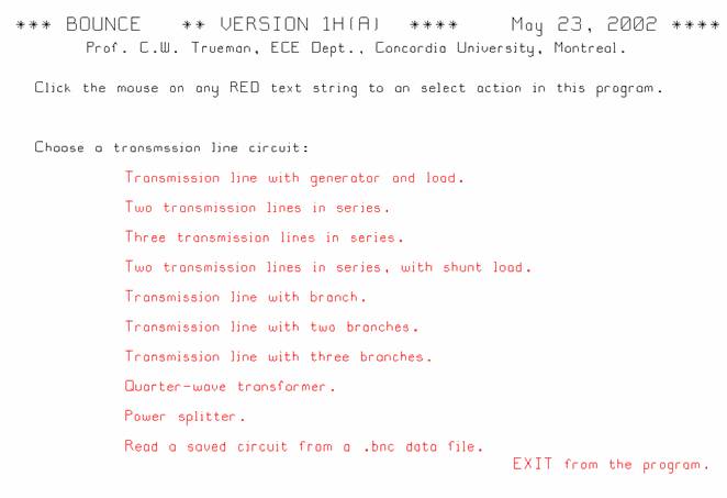
Fig. 1 The entry menu lets the user choose a circuit template.
BOUNCE has a variety of built-in "circuit templates" of increasing complexity, from a simple transmission line to a line with three branches. Choose a circuit template by clicking the mouse on the name of the circuit. Or you can recall a previously saved circuit by choosing “Read a saved circuit…”, which reads a “bnc” file or “bounce” file from the disk.
To solve your circuit, enter your component values using the menus for the generator, the transmission lines, and the loads, as described below. You can save the circuit as a “bnc” file. Then when you re-start BOUNCE you can read the circuit into BOUNCE so that you can carry on with your work without re-entering the circuit values.
The “EXIT” button at the lower right on this menu terminates the program.
3 BOUNCE’s Main Menu
Choose a circuit template in the entry menu, and BOUNCE sets up the circuit and then shows the main menu. For example, choosing "transmission line with generator and load" by clicking the mouse on the red text string obtains the main menu shown in Fig. 2.

Fig. 2 The main menu in BOUNCE shows the circuit schematic and lets the user choose the generator, line properties and load properties, then run the simulation.
The main menu
has four parts. The center of the screen shows a schematic of the circuit
template. Here we see a voltage generator ![]() , with it internal resistance
, with it internal resistance ![]() , a
transmission line labeled "#1" at the bottom center, and a load
, a
transmission line labeled "#1" at the bottom center, and a load ![]() . BOUNCE uses
"voltmeters" to measure the voltage as a function of time at selected
points on the transmission line. In this circuit, there is a
"voltmeter"
. BOUNCE uses
"voltmeters" to measure the voltage as a function of time at selected
points on the transmission line. In this circuit, there is a
"voltmeter" ![]() near the center of the transmission line.
You can move this voltmeter and add more with the voltmeters menu, which is
described below.
near the center of the transmission line.
You can move this voltmeter and add more with the voltmeters menu, which is
described below.
In the lower right-hand corner, there is a “GO” button and an “EXIT” button. Clicking the mouse on “GO” runs the simulation and so shows the voltage wave traveling along the transmission line. Clicking “EXIT” terminates the BOUNCE program.
The top area of the main menu has buttons that you can click to modify the properties of the generator, of each transmission line in the circuit, and of each load in the circuit. These are described more fully below. The area below the circuit diagram offers menu items to modify the time step and the length of the time cycle; to change the generator; to move the voltmeters; to view the current or the positive-going and negative-going traveling wave components; to save the circuit as a “bnc” file; and to change to a new circuit. These are called the “Program Control Buttons”.
4 Program Control Buttons
Below the circuit diagram on the main menu, there are seven “program control buttons”, as follows.
Choose the time step: Click
the mouse on “choose the time step” in the main menu of Fig. 2 to get the time
step menu of Fig. 3. BOUNCE divides time into “time steps” of length ![]() . Each
transmission line is divided into cells of length
. Each
transmission line is divided into cells of length ![]() where
where ![]() is the phase velocity
or wave speed on the transmission line. The length of each transmission line
is approximated with integer numbers of cells. Thus the lengths used in the
simulation are not exact, but instead are rounded to the nearest integer number
of cells. Thus BOUNCE does not obtain the exact solution to the transmission
line problem. Instead, BOUNCE approximates the lengths of the transmission
lines and so obtains an approximate solution. Typing or clicking the mouse on
F1 lists the true lengths and the approximate lengths that BOUNCE will use. If
you use a coarse time step, the lengths of the lines are quite approximate but
the simulation proceeds rapidly. If you use a fine time step, the length
approximation is more accurate but the simulation goes slowly. If the total
number of transmission line cells is 100 to 200, we get reasonable accuracy and
speed. BOUNCE "runs" the simulation for a "cycle" of time
steps then pauses so that you can look at the result.
is the phase velocity
or wave speed on the transmission line. The length of each transmission line
is approximated with integer numbers of cells. Thus the lengths used in the
simulation are not exact, but instead are rounded to the nearest integer number
of cells. Thus BOUNCE does not obtain the exact solution to the transmission
line problem. Instead, BOUNCE approximates the lengths of the transmission
lines and so obtains an approximate solution. Typing or clicking the mouse on
F1 lists the true lengths and the approximate lengths that BOUNCE will use. If
you use a coarse time step, the lengths of the lines are quite approximate but
the simulation proceeds rapidly. If you use a fine time step, the length
approximation is more accurate but the simulation goes slowly. If the total
number of transmission line cells is 100 to 200, we get reasonable accuracy and
speed. BOUNCE "runs" the simulation for a "cycle" of time
steps then pauses so that you can look at the result.
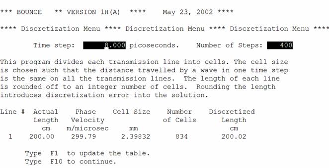
Fig. 3 The time step menu.
The time-step menu is shown in Fig. 3. Enter a time step in the box at the top left, and enter the number of time steps per cycle at the top right. Then hit F1 to update the table at the bottom of the screen. This shows the true length of each transmission line at left, the wave speed, the cell size, the number of cells, and the approximate length of the line that the program will use, at right. For the example shown above, the time step is 8 ps, and the 2-m transmission line is approximated with 834 cells of 2.39832 mm length. Thus the 200 cm actual length is approximated as 200.02 cm.
The time step is an effective speed control for the animation. BOUNCE was written on a 266 MHz Pentium and the animation can be seen effectively with a total of about 200 cells on all the transmission lines. On an 1266 MHz Pentium, the animation is too fast and the time step needs to be reduced to about 1/4 of the value, so that there are about 800 cells total to obtain an effective animation speed.
The number of time steps in a time cycle is chosen to be 400 in Fig. 3. BOUNCE runs the simulation for 400 time steps, or one time cycle, then pauses to let you examine the screen. You can use the mouse to “read back” the value of the voltage at any location, as described below.
Choose the number of time steps per cycle: This is a separate menu that lets you set the number of time of steps per cycle quickly.
Choose the generator: This button gets the same menu as the "Generator" button at the top of the screen. Choose the type of source: step, pulse, triangle, square wave or "pulse train", or sinusoid. Note that you must be careful that your pulse length makes sense compared to the delay times of your transmission lines, and to the time step that you have chosen. As in any computer simulation, it is easy to compute nonsense!
Place a voltmeter: This menu lets you choose the places on the transmission lines where you are measuring the voltage as a function of time. It is described more fully below. You can have up to four voltmeters.
Draw the current on each transmission line: When the simulation is run by clicking the mouse on the "GO" button at the lower right, BOUNCE draws the voltage on each transmission line as a function of the position on the line, at each time step. As time advances the voltage wave progresses across the screen and is reflected from junctions and loads. To see the current wave on the transmission lines as well, click the “Draw the current” button. The voltage wave is drawn in blue, and the current in red.
Draw the incident and
reflected voltage waves: Clicking the "GO" button shows the
voltage on the transmission lines as a function of distance and time. The
voltage can be written as the superposition of a positive-going traveling wave ![]() plus a
negative-going traveling wave,
plus a
negative-going traveling wave, ![]() according to
according to
![]()
Sometimes it is instructive to
see the positive-going wave and the negative-going wave individually. Clicking
the “Draw the incident…” button and the program draws the incident wave ![]() and the
reflected wave
and the
reflected wave ![]() individually, as well as their sum.
individually, as well as their sum.
Save the circuit: If you have entered values for the generator, the line lengths, speeds and characteristic resistances, and values for the loads, then you may want to save all these values to a "bnc" data file. Then you can recall the circuit later and you won’t have to re-enter all the numbers. You can do this using the “Save the circuit” menu button. Enter a path name and a file name in the menu boxes. The standard file extension for this program is "bnc".
Choose a new circuit: This button gets back the entry menu, which lists the circuit templates, and also lets you read a circuit from a "bnc" file.
5 Running the Simulation
The “default” values for the simple circuit of Fig. 1 are as follows. The generator is has internal resistance 50 ohms and the open-circuit voltage is a 10-volt, 0.5-ns pulse. The transmission line has length 2 m, propagation velocity 29.797 cm/ns, and characteristic resistance 50 ohms. The load is 50 ohms, matched to the transmission line.
Clicking the mouse on the “GO” button in the main menu obtains the simulation menu and starts time advancing. With the time step set to 8 ps and the time cycle set to 400 steps, the program pauses after 3.2 ns and the display is shown in Fig. 4. The pulse from the generator advances onto the transmission line and propagates about a quarter of the distance to the load.
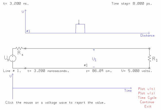
Figure 4 A pulse traveling on the simple transmission line circuit.
The simulation menu shown in Fig. 4 has three parts. The graph at the top of the screen in Fig. 3 shows voltage as a function of distance along the transmission line. The generator launches a wave onto the transmission line, and as time advances, you see the wave traveling along on the transmission line. The graph across the bottom of the screen shows voltage as a function of time at the voltmeter locations on the transmission line. In Fig. 3, the pulse has not yet reached the voltmeter so the voltage there is zero. The simulation menu of Fig. 3 shows the time step in the upper right corner to remind the user that BOUNCE advances time in discrete steps, and the results obtained can be dependent on the time step.
Click the mouse on the voltage pulse at the top of the screen to “read back” the voltage and position. Fig. 4 shows that the BOUNCE program draws a small arrow on the waveform at the location where the mouse was clicked, and reports the value of the time, position and voltage below the circuit schematic. Thus, in Fig. 4, at time-3.2 ns and 86.09 cm distance, the voltage is 5.000 volts.
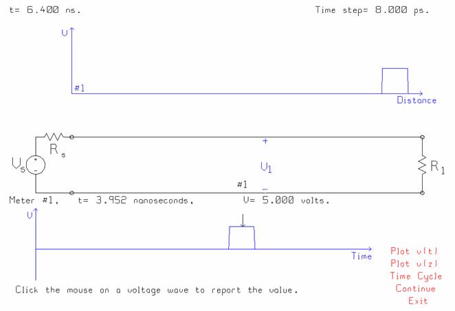
Fig. 5 The simulation after one more time cycle.
As time advances the leading edge of the voltage launched from the generator passes the voltmeter location, and the voltage steps up from zero on the voltage-vs.-time graph. Thus, if we click “Continue” in Fig. 4, BOUNCE advances time for another time cycle of 400 steps, and the pulse travels across the screen to a location near the load. As the pulse goes by the V1 voltmeter location, the voltage steps up in the voltage-vs-time graph across the bottom of the screen. Click the mouse on voltage pulse to “read back” the voltage and time, and BOUNCE reports the time and voltage below the circuit schematic. The “read back” feature is very handy for finding the values of reflected pulses at loads and transmitted pulses at junctions!
The simulation menu of Fig. 4 and Fig. 5 has some buttons at the lower right to determine what the program will do next. “Plot v(t)” and “Plot v(z)” draw neatly-labeled rectangular graphs of the voltage as a function of time and distance, respectively, and are described in the next section. "Time Cycle" gets a menu that lets you increase or decrease the number of steps in each time cycle, and continue the simulation for another time cycle. "Continue" tells the program to continue the simulation for another time cycle, then pause once again. "EXIT" returns to the main menu.
BOUNCE was written on a 266 MHz Pentium computer and the animation speed was good with about 200 cells in total on all the transmission lines. More modern computers run at much higher speeds so more, smaller cells can be used and the animation speed is fast enough to be effective. Thus on a 1266 MHz Pentium the 834 cells used for Fig. 4 and 5 shows the wave traveling at a reasonable speed across the computer screen.
By choosing a short time cycle we can watch the voltage wave advance with frequent pauses. During each pause, we can use the mouse to “read back” values from the curves. Advancing time in short cycles permits the amplitude of reflected waves to be read back after each individual reflection. Conversely, choosing a long time cycle shows the overall picture of what happens in the circuit, with many reflections leading to steady state. Both a short and a long time cycle are useful ways of studying the behavior of the circuit.
6 Graphing the Transmission Line Voltage as a Function of Distance or Time
The simulation menu has buttons labeled “Plot v(z)” and “Plot v(t)” to graph the voltage on each transmission line as a function of distance and of time, respectively. The graphs are more formal and better labeled than those on the simulation menu.
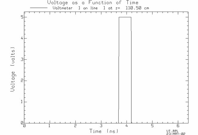
Fig. 6 The voltage at the voltmeter location V1 as a function of time.
If you click “Plot v(t)” in Fig. 5, then BOUNCE writes the voltage at each voltmeter location to a file called “vt.rpl” and starts the rectangular-plotting program called RPLOT to draw the graph. You can adjust the size of the axes and change the labels, and so forth, to make a graph suitable for a lab report or homework assignment. In RPLOT you can click the mouse on the curve and the program will “read back” the value and report it in the lower left corner of the screen. If there are several voltmeters RPLOT will display all the curves on the same graph. You can select just one of the curves with F1 then F4. You can control the line time and the text of the legend with F9. If you display only one curve on the graph, tou can write the data for that curve to a “two column” data file with F1 then F7, and then use your favorite plotting program to draw the graph.
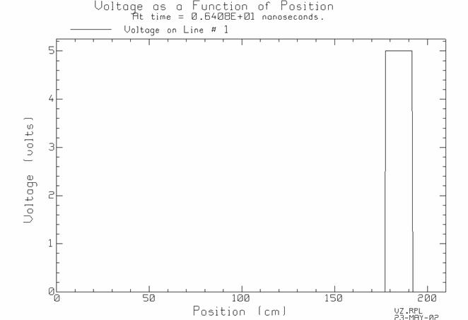
Fig. 7 The voltage on the transmission line as a function of distance.
To graph the voltage on the transmission line as a function of the distance at time = 6.4 ns, click the mouse on “Plot v(z)” in Fig. 5. BOUNCE creates file “vz.rpl” and starts RPLOT to graph it, resulting in the drawing of Fig. 7. Unfortunately there is no user’s guide for RPLOT so you need to try the various function keys to discover the program’s features!
7 Generator, Line and Load Menus
The main menu of Fig. 2 offers sub-menus across the top of the screen for the “Generator”, for each “Line” and for each “Load”. This section describes these menus for choosing the generator, the properties of the transmission lines, and the load properties.
7.1 Generator Menu
The “generator menu” lets the user change the properties of the generator, and is obtained by clicking the mouse on “Generator” at the top of the main menu.
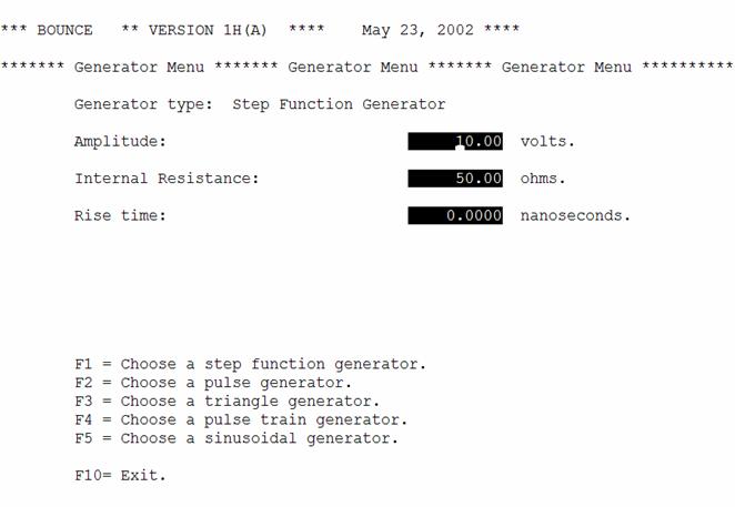
Fig 8 The generator menu, showing the menu items for a step generator.
The generator menu of Fig. 8 offers five types of generator: a step function, a pulse function, a triangle function, a pulse train and a sinusoid. The following describes the parameters of each type of generator.
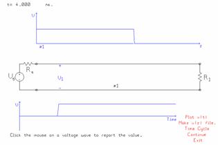
Fig. 9 The voltage waveform of the step generator.
Type F1 to select a step function generator, and then enter the amplitude or open-circuit voltage, and the internal resistance, in the menu boxes. The step function generator’s waveform is shown in Fig. 9. Even if the rise time is zero, the step generator takes one time step to rise linearly from zero to its full amplitude so is not a true mathematical “step function”. A longer “rise time” can be specified. The voltage rises linearly from zero to the full amplitude in the rise time. Type F10 to return to the main menu.
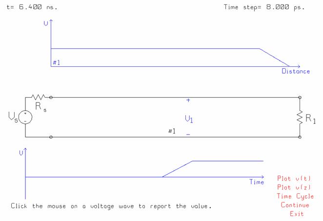
Fig. 10 A step with an 800 ps rise time.
Fig. 10 shows the “step generator” function when the rise time is set to 800 ps with a time step of 8 ps. The “step” is actually a ramp function that increases linearly from 0 to 5 volts in 800 ps.
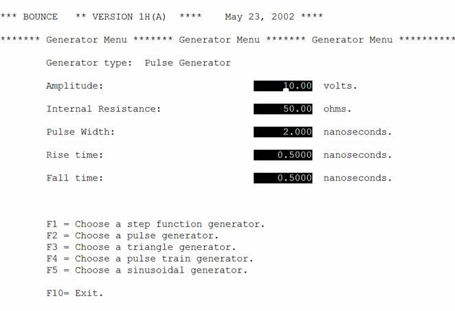
Fig. 11 The pulse generator menu.
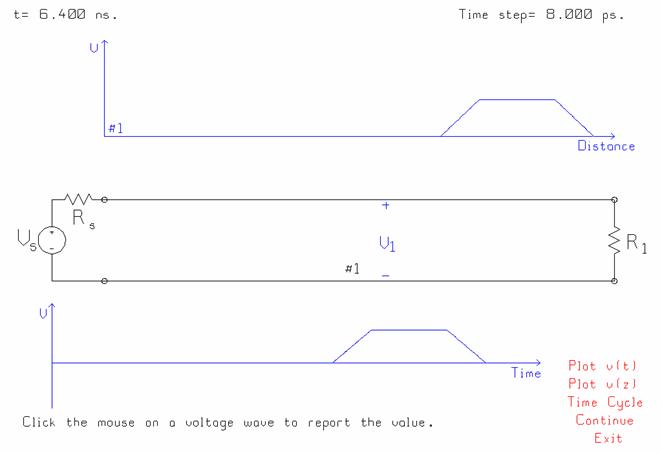
Fig. 12 A pulse of length 2 ns with a rise time of 0.5 ns and a fall time of 0.5 ns.
Fig. 11 shows the pulse generator menu. To define the pulse, the user must specify the amplitude of the pulse and internal resistance of the generator. In addition, the user must specify the length of the pulse, the rise time and the fall time. In Fig. 11 the overall length is 2 ns, the rise time is 0.5 ns and the fall time is 0.5 ns. Fig. 12 shows that the pulse rises linearly from zero to five volts in 0.5 ns, stays at 5 volts for 1 ns, and then falls linearly from 5 to 0 volts in 0.5 ns, for an overall length of 2 ns. The minimum rise time and fall time can be entered as zero to get the sharpest possible pulse. The actual minimum is one time step for the rise time and one time step for the fall time.
Note that if the generator has a 50 ohm internal resistance and a 10 volt open circuit voltage, and the transmission line has a 50 ohm characteristic resistance, then the voltage divider relation at the generator terminals determines that the pulse launched onto the transmission line will have an amplitude of 5 volts.
The pulse shown above has a physical length of about one-quarter the length of the transmission line. The pulse length can be set much shorter than the transmission line length but should not be shorter than one time step. Short pulses are used to model situations in which the propagation time on the transmission lines is much longer than the pulse length. Conversely, the pulse length can be much longer than the transmission line length, useful for demonstrating effects in digital circuits with short interconnections, but longer than the usual limit for the use of lumped circuit analysis[3].
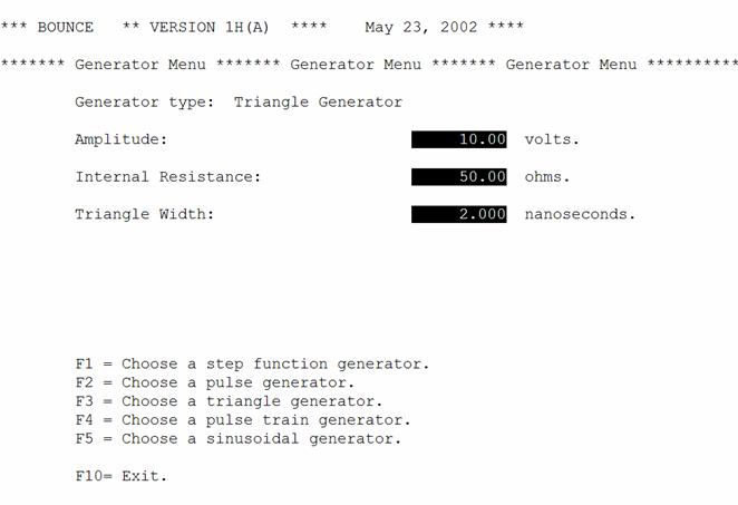
Fig. 13 The triangle generator menu.

Fig. 14 The triangle generator’s waveform.
The third generator choice is the triangle function, with the menu in Fig. 13. Fig. 14 shows that the triangle rises linearly from zero to the overall amplitude, then falls back to zero in one time step. The pulse is useful for demonstrating that the voltage as a function of distance on the transmission line is reversed compared to the voltage as a function of time, as Fig. 14 shows. This triangle function could be obtained using the rise time and fall time parameters for the pulse described above. It is convenient to have the triangle available as a separate “built-in” function.
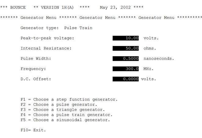
Fig. 15 The pulse train menu.
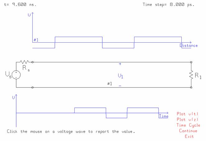
Fig. 16 The voltage waveform for the pulse train.
Fig. 15 shows the pulse train menu, which requires five parameters. The peak-to-peak swing of the pulse train is specified as 10 volts, and the internal resistance of the generator as 50 ohms. The length of time that the pulse is “on” is specified, at 2 ns for the diagram shown above. The frequency of the pulse train must be given. For the diagram above, the period was chosen as 2 ns and the frequency 300 MHz, for a period of 3.333 ns, so the pulse is “off” for 1.333 ns. Zero D.C. offset was specified so the pulse is symmetrical about the zero volts axis. If a 5 volt offset is specified, then the pulse will vary from zero volts to 10 volts. The rise time and fall time are 1 time step and cannot be changed.
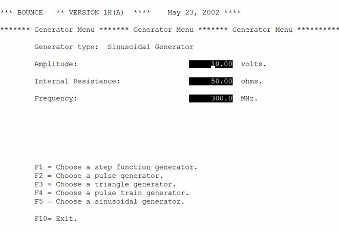
Fig. 17 The menu for the sinusoidal generator.
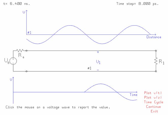
Fig. 18 The sinusoidal generator’s waveform.
The fifth generator is a sinusoid. Fig. 17 shows the menu for specifying the amplitude, internal resistance, and frequency. Fig. 18 shows the waveform. The generator turns on abruptly. The sine wave generator is used to investigate the transients on the transmission line as the leading edge of the sinusoid is reflected from junctions between transmission lines and from loads. As time goes by the transmission line circuit will reach the sinusoidal steady state, and the steady state response of the circuit will be calculated by BOUNCE.
7.2 Transmission Line Menu
The transmission line menu lets you set the parameters of one of the transmission lines in the circuit. Click the mouse on “Line #1” to set the properties of transmission line number one.
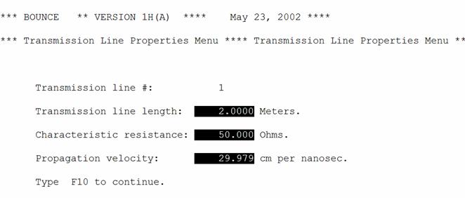
Fig. 19 The transmission line menu.
The menu for the transmission line parameters is shown in Fig. 19. It requires that the length of the transmission line be entered, and the characteristic resistance, and the speed of propagation or phase velocity. Note that in BOUNCE the transmission lines are lossless.
7.3 Load Menu
The load menu lets you choose the circuit for each load on the transmission line, and specify the value of the components. There are two kinds of loads. The first kind is a “shunt load” connected between transmission lines. This kind of load must be a resistor, with no inductance or capacitance. BOUNCE calls this a “Resistive” load. The second kind of load is a load that terminates a transmission line. This can be a simple resistor, or a series connection of a resistor and a capacitor, or a parallel resistor and capacitor, or a series inductor and resistor, or a parallel inductor and resistor. Thus there are five configurations for the load terminating any transmission line.
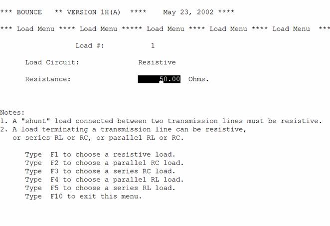
Fig. 20 The load menu.
Fig. 20 shows the load menu. Function keys F1 to F5 choose the type of load. A load that is connected at the junction of two transmission lines must be resistive. (Why? BOUNCE is not programmed with an algorithm for reactive loads connected between two lines.) A load terminating a transmission line can be a simple resistor (type F1); a parallel connection of a resistor and a capacitor (type F2); a series connection of a resistor and a capacitor (type F3); a parallel connection of a resistor and an inductor (type F4); or a series connection of a resistor and an inductor (type F5). In Fig. 20 the simple resistor has been chosen and the menu provides a box for entering the value.
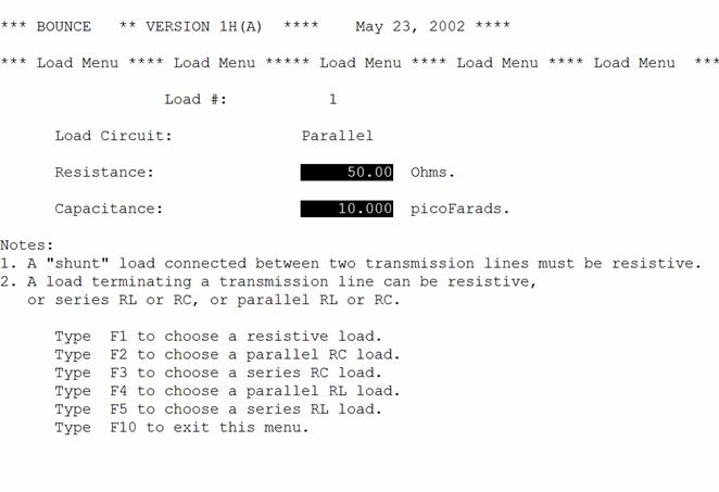
Fig. 21 The load menu for a parallel RC load circuit.

Fig. 22 The parallel RC load circuit.
Fig. 21 shows the load menu when the parallel RC load is chosen, to obtain the load circuit of Fig. 22. Enter the value of the resistor and the capacitor. The initial voltage across the capacitor is zero volts. For a simple capacitive load, Fig. 23, make the value of the resistor very large, say 1 million ohms. Parallel RC loads are used to model the input of CMOS gates in switching circuits.
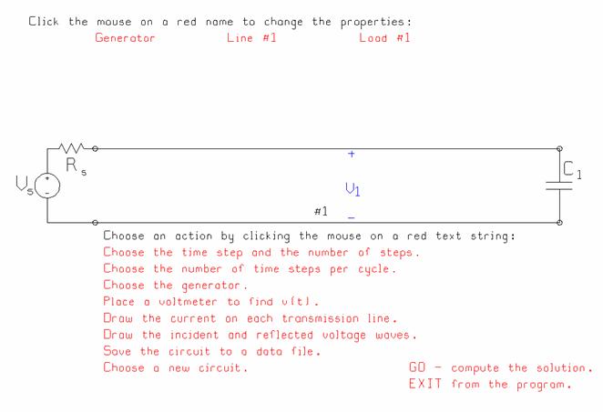
Fig. 23 A simple capacitive load can be obtained with the parallel RC load circuit by setting the value of the resistor to 1,000,000 ohms.
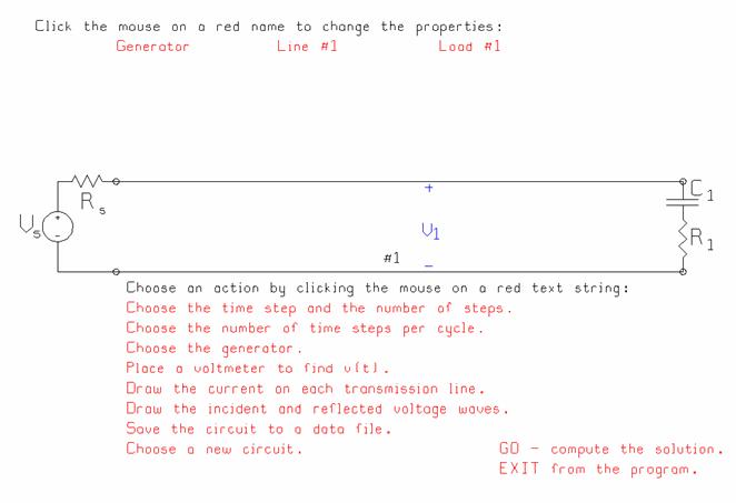
Fig. 24 The series RC load circuit.
Fig. 24 shows the series RC load circuit. The initial voltage across the capacitor is zero volts. Specify the value of the resistor and the capacitor in the load menu. For a simple capacitive load, make the value of the resistor zero.
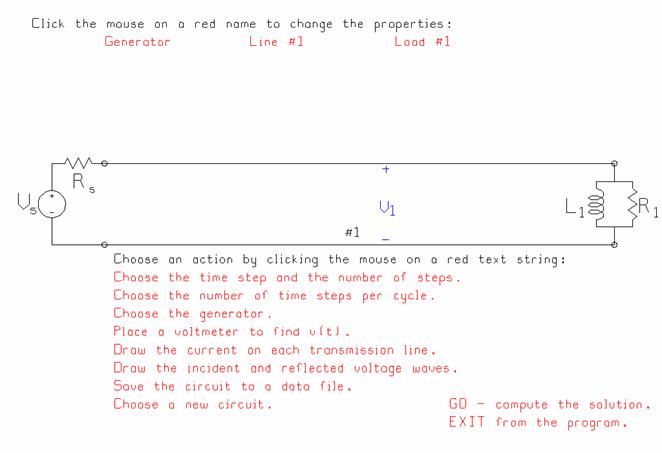
Fig. 25 The parallel RL load circuit.
Fig. 25 shows the parallel RL load circuit. The load menu provides boxes for entering the value of the resistor and the inductor. The initial current through the inductor is zero amps. For a simple inductive load, with no resistor, make the value of the resistor very large, say 1 million ohms.
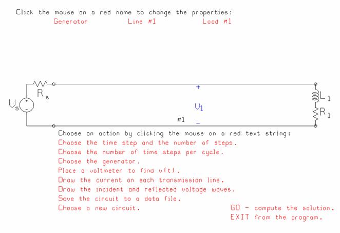
Fig. 26 The series RL load circuit.
Finally, the last load type is the series RL load of Fig. 26. Enter the value of the resistor and the inductor in the load menu. The initial current through the inductor is zero amps. For a simple inductor, make the value of the resistor zero, to obtain the load of Fig. 27.
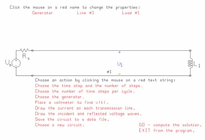
Fig. 27 A circuit with a simple inductive load, consisting of the series RL load circuit with the resistor set to zero.
8 Voltmeter Setup Menu
In BOUNCE, placing a “voltmeter” on a transmission line is like connecting an oscilloscope across the circuit at that location. The program reports the voltage as a function of time at the voltmeter’s location.
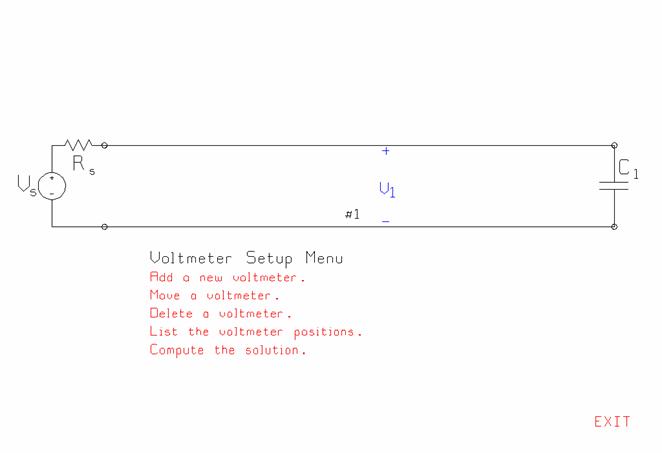
Fig. 28 The voltmeter setup menu.
The voltmeters setup menu, Fig. 23, lets you position a "voltmeter" anywhere in the circuit, so you can find the voltage as a function of time anywhere in the circuit. You can have as many as four voltmeters. These are color-coded so that you can see which curve corresponds to each voltmeter location. A larger, clearer graph of the voltage at each voltmeter as a function of time is obtained by clicking the mouse on the "Plot v(t)" button in the simulation menu of Fig. 3. Clicking “make a v(t) file” creates an “rpl” file, which can be graphed with the rectangular-plotter program “RPLOT”.
The voltmeter setup menu of Fig. 28. has five buttons for adding a voltmeter, moving a voltmeter, deleting one, listing their locations, and then starting the simulation, as follows.
“Add a new voltmeter” is used to put another voltmeter into the circuit. Click the mouse on “Add a new voltmeter”, then click the mouse on the place in the circuit where you want to put the voltmeter. A new voltmeter simulation appears. You can have up to four voltmeters.

Fig. 29 A circuit with three voltmeters.
In the circuit of Fig. 29, the user has added two new voltmeters. V2 measures the voltage at the input to the transmission line, and V3 measures the voltage at the load. Note that the “V3” label on the schematic overlaps the symbol for the load capacitor, an unavoidable problem if the voltmeter is to be drawn at its true location on the transmission line.
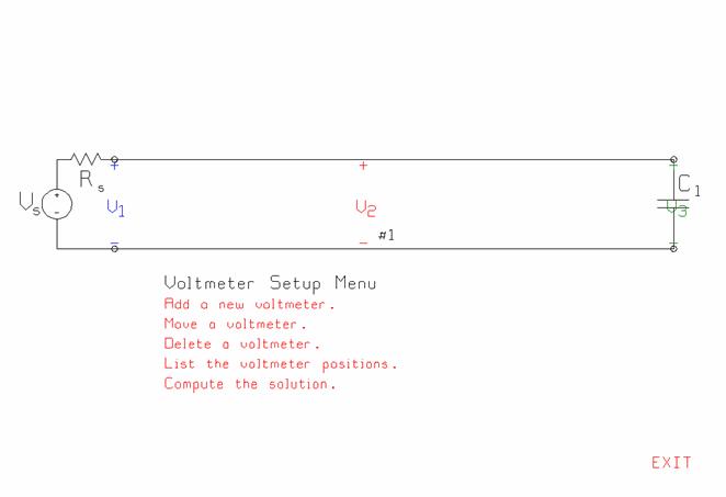
Fig. 30 The “move” function has been used to move V1 to the generator terminals and V2 to approximately the middle of the transmission line.
“Move a voltmeter” lets you change the position of any voltmeter. Click the mouse on “Move a voltmeter”. If there is only one voltmeter, click on the new location for the voltmeter. If there are two or more, first click “Move a voltmeter” then click the mouse on the voltmeter that you wish to move. Then click on the new location. In Fig. 30, the set of three voltmeters of Fig. 29 has been adjusted by moving V2 to a position approximately at the middle of the transmission line, and moving V1 to the generator terminals.
“Delete a voltmeter” lets you remove a voltmeter from the circuit. Click “Delete a voltmeter” then click on the voltmeter you wish to remove.
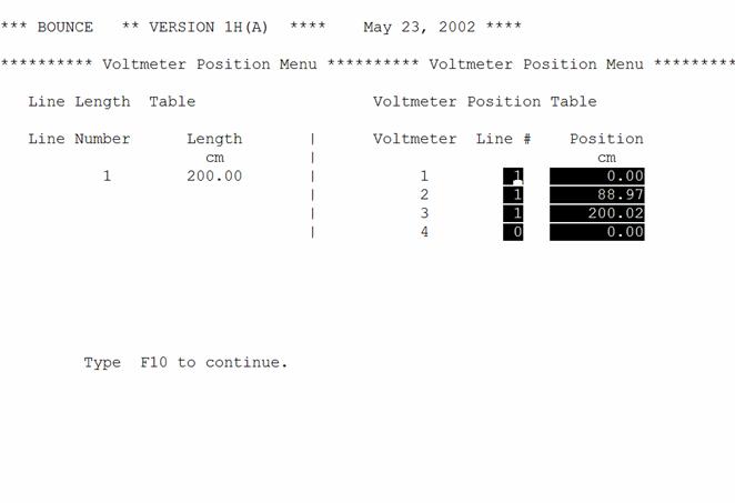
Fig. 31 The “list” menu permits you to precisely position the voltmeters on the transmission lines.
“List the voltmeter locations” gets the menu of Fig. 31, which gives you a tabulation of where the voltmeters are located in the circuit. At left there is a list of the transmission lines and their overall lengths. At right, there is a list of the voltmeters, the line on which each voltmeter is positioned, and the location on that line. Voltmeter #1 is at location 0 cm on line #1. Voltmeter #2 is at 88.97 cm on the line, which is 200 cm long. Voltmeter #3 is at 200.2 cm, which reflects the approximation of the line lengths discusses in conjunction with Fig. 3.
You can change the locations by typing new values into the fields of the menu. This is good for precisely positioning voltmeters in the circuit. In Fig. 31, the position of voltmeter #2 can be changed to 100 cm to put this voltmeter exactly at the center of the 2 m transmission line. Note that you can add a 4th voltmeter to the circuit by entering the line number and position for the 4th meter into the boxes at the lower right of this menu. You can also delete a voltmeter by entering “0” for the transmission line on which it is located.
The last two buttons in the menu of Fig. 30 are "Compute the solution", which runs the simulation, and "EXIT", which returns to the main menu.
9 Drawing the Current Waveform
Sometimes the current on the transmission line is of interest in understanding the behavior. To see the current on each transmission line as a function of distance, as well as the voltage, click the mouse on the button “Draw the current…” in the main menu of Fig. 2. For example, consider a transmission line driven with a step generator of height 10 volts and internal resistance 50 ohms. The transmission line is 2 m in length and has characteristic resistance 50 ohms. The speed of propagation is equal to the free-space speed of light, 29.979 cm/ns. The load is a 10 pF capacitor. Position a voltmeter at load, as shown in Fig. 32.
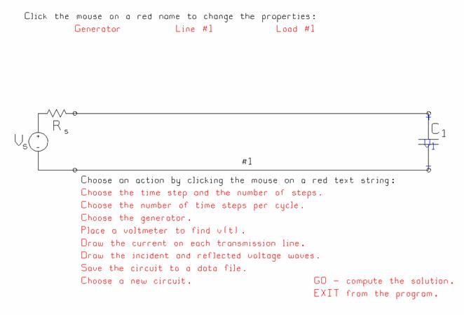
Fig. 32 A circuit with a 10 pF capacitor as a load, and a voltmeter in the middle of the line.
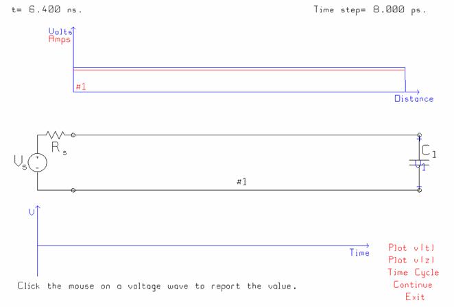
Fig. 33 The voltage and current on the transmission line as a function of distance at t=6.4 ns.
Running the simulation until t=6.4 ns obtains the voltages and currents shown in Fig. 33. At the top of the figure we have the voltage on the transmission line as a function of distance, blue curve, and the current as a function of distance, red curve. The leading edge of the step function has progressed almost as far as the load. The voltage at the V1 voltmeter is still zero because the step function has not yet reached the load.
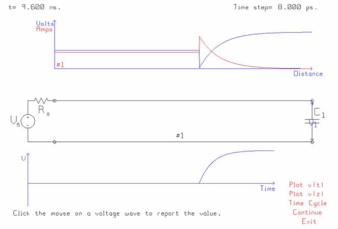
Fig. 34 The voltage and current at 9.6 ns.
Letting the time advance to 9.6 ns obtains the
response in Fig. 34. The top graph shows the voltage in blue and the current
in red. The bottom graph shows the voltage at the load, V1, as a function of
time. When the step function’s leading edge reaches the capacitor, the initial
voltage is zero. The capacitor cannot charge instantaneously, so it pulls the
transmission line voltage down to zero when the leading edge of the step first
arrives. Then the capacitor gradually charges, and the voltage rising
exponentially towards the final value of 10 volts, because the capacitor
behaves as an open circuit as time gets large. The exponentially-rising
waveform is reflected from the capacitive load towards the generator, and so in
the voltage-vs.-distance graph at the top, we see the blue curve stepping down
to 0 volts and then charging exponentially to 10 volts. Conversely, the
initial value of the current is large, equal to the 5-volt step with a 50 ohm
resistance working into a short circuit. As the capacitor charges the voltage
across it gradually increases, and the current gradually decreases towards a
final value of 0 amps. The time constant of the exponential changes is ![]() 50 ohms x 10
pF = 50 ps. After about five time constants, the capacitor is fully charged
and behaves as an open circuit. The final value of the voltage across the
capacitor is then 10 volts.
50 ohms x 10
pF = 50 ps. After about five time constants, the capacitor is fully charged
and behaves as an open circuit. The final value of the voltage across the
capacitor is then 10 volts.
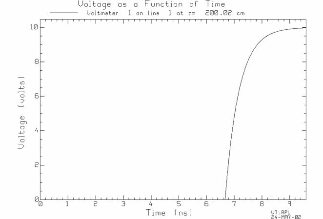
Fig. 35 The voltage and current waveforms after 12.8 ns.
To verify the time constant, click the mouse on “Plot v(t)” to get the voltage-vs.-time graph for voltmeter V1, shown in Fig. 35. The voltage increases exponentially from 0 to 10 volts, starting at t=6.672 ns. After one time constant, the voltage is 10(1-1/e)=6.321 volts. Use the “read back” feature in RPLOT to find the time when the voltage is close to 6.321 volts, which is 7.176 ns. The time constant is (7.176-6.672)=50.4 ps, close to the expected value of 50 ps. You can also “read back” the needed values directly from the simulation menu of Fig. 34.

Fig. 36 The voltage and current waveforms after 12.8 ns.
It is instructive to put the voltmeter at the centre of the transmission line, to obtain the voltage curve in Fig. 36. Allowing the time to advance to 12.8 ns lets the reflection propagate past the voltmeter location, reflect from the capacitor, and then propagate back past the voltmeter. The voltage at V1 initially steps up to 5 volts as the leading edge of the generator’s voltage goes past the center of the transmission line. The voltage remains at 5 volts until the reflection from the capacitor arrives at the V1 location. Then the voltage steps down to 0 volts, and then rises exponentially towards the final value of 10 volts.

Fig. 37 The voltage on the transmission line as a function of position.
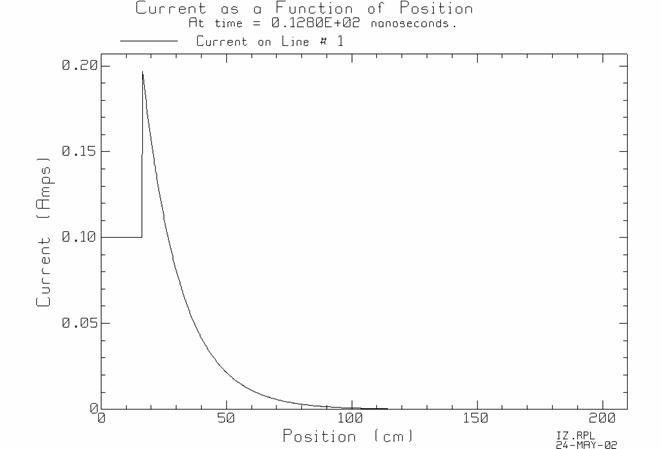
Fig. 38 The current as a function of position on the transmission line.
When BOUNCE is set up to plot the current, then clicking “Plot v(z)” obtains both the voltage on the transmission line as a function of position, Fig. 37, and the current as a function of position, Fig. 38. These are drawn in separate RPLOT windows and saved in “rpl” files “VZ.RPL” and “IZ.RPL”, respectively.
10 Viewing the Incident and Reflected Voltage Waveforms
Sometimes it is useful to decompose the voltage on the transmission line into the “incident” or positive-going voltage wave and the “reflected” or negative-going voltage wave. Thus the voltage on the transmission line can be decomposed as
![]()
where the incident wave is ![]() and the
reflected wave is
and the
reflected wave is ![]() individually. Click the mouse on “Draw
the incident and reflected voltage waves”, and the program will draw the
functions for the incident wave
individually. Click the mouse on “Draw
the incident and reflected voltage waves”, and the program will draw the
functions for the incident wave ![]() and the reflected wave
and the reflected wave ![]() individually,
as well as their sum. Two examples will be presented. In the first a pulse is
partially reflected from a junction and partially transmitted. The second
example will be the reflection of a sinusoidal voltage from an unmatched load.
individually,
as well as their sum. Two examples will be presented. In the first a pulse is
partially reflected from a junction and partially transmitted. The second
example will be the reflection of a sinusoidal voltage from an unmatched load.
10.1 Reflection and Transmission at a Junction
Consider a circuit with two transmission lines in series, shown in Fig. 40. The generator has internal resistance 50 ohms, and the open-circuit voltage is a 10 volt pulse lasting 0.5 ns. Line #1 is 1.5 m in length, with characteristic resistance 50 ohms, and speed of propagation 30 cm/ns. Line #2 is 1 m in length with characteristic resistance 100 ohms, and speed of propagation 30 cm/ns. The load is 100 ohms. Choose a time step of 10 ps. Position voltmeter #1 at 130 cm on line #1, 20 cm from the junction. Position voltmeter #2 at 10 cm on line #2. The voltmeters will be used to observer the reflected pulse from the junction and the transmitted pulse through the junction. Also, to separate the incident pulse and the reflected pulse on line #1, click the mouse on “Draw the incident and reflected voltage waves”.
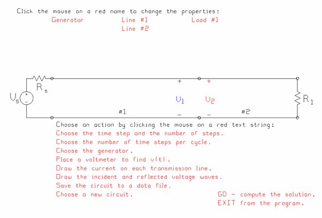
Fig. 39 A transmission line circuit with two lines in series.
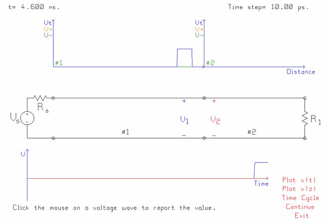
Fig. 40 Two transmission lines in series.
Fig. 39 shows the transmission line circuit. Time has been advanced to 4.6 ns in steps of 10 ps. The incident pulse amplitude is 5 volts, and the leading edge has reached the location of the V1 voltmeter, where the voltage has stepped up to 5 volts. When the pulse reaches the junction we expect to see a reflected pulse of amplitude 5x(100-50)/(100+50)=1.333 volts, and a transmitted pulse of amplitude 5x( 2x100 ) / (100+150) = 6.667 volts.
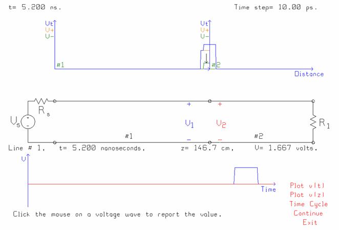
Fig. 41 Time has advanced to 5.2 ns and the reflection and the junction is in progress.
Allow time to advance to 5.2 ns, permitting the leading edge of the pulse to reach the junction, and partial reflection and transmission to take place. Fig. 41 shows the voltages on the transmission lines. The red curve on line #1 shows the incident pulse, of amplitude 5 volts. The green curve shows the reflected pulse, and by clicking the mouse on the green curve, we can “read back” the value as 1.667 volts. The sum of the red and the green curve is the “total” voltage on line #1, given by the blue curve. This is 5+1.667 volts or 6.667 volts. On line #2, there is no reflected pulse, only a transmitted pulse. The amplitude of the transmitted voltage is 6.667 volts as expected.
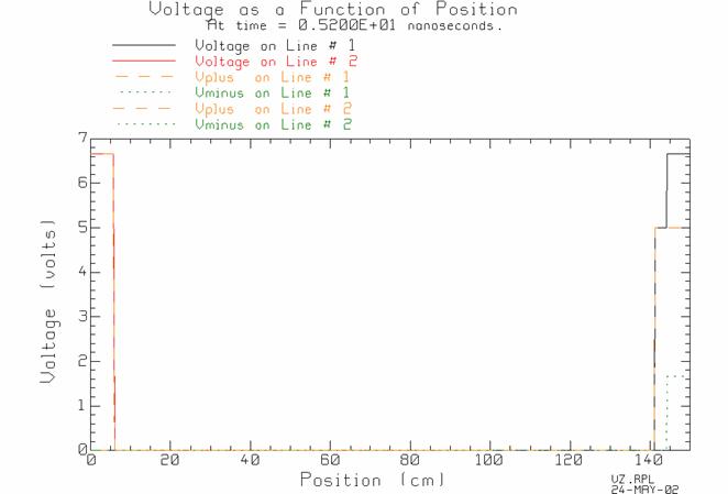
Fig. 42 The voltages on the two transmission lines at 5.2 ns.
To obtain a rectangular graph of the voltages as functions of distance, click the mouse on “plot v(z)” in Fig. 41. This runs RPLOT and graphs the voltages as in Fig. 42. The curves show the “total” voltage on line #1 as as solid black curve, and the voltage on line #2 as a solid red curve. The voltages are decomponsed into the “positive going” wave, Vplus, and the “negative going” wave, Vminus, on each line. Thus on line #1, the positive-going pulse is a long-dashed red curve at the right side of the graph, and the negative-going wave is a short-dashed green pulse of height 1.667 volts, at the right side of Fig. 42. RPLOT can be used to separate the six curves, and graph any of them separately. Thus, using F1 then F4 in RPLOT, and choosing only Vplus and Vminus on line #1, obtains Fig. 43.
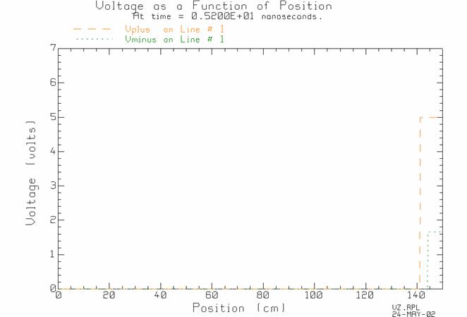
Fig. 43 The positive-going wave and the negative-going wave on line #1.
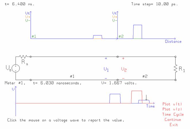
Fig. 44 The voltages on the transmission lines at 6.4 ns.
If time is permitted to advance to 6.4 ns, the voltages of Fig. 44 are seen. The reflected pulse has propagated past the location of the V1 voltmeter, and in the blue curve at the bottom of the computer screen we seen the incident pulse at V1, of amplitude 5 volts, and the reflected pulse, of amplitude 1.667 volts. The red curve is the transmitted pulse, of amplitude 6.667 volts. You can click the mouse on “plot v(z)”
10.2 Reflection of a Sinusoid at an Unmatched Load
The second example using decomposition into the positive-going and negative-going traveling waves concerns the reflection of a sinusoid at an unmatched load. Choose the simple transmission line circuit in the entry menu of Fig. 1. Set the generator to a 10-volt, 300 MHz sine wave with internal resistance 50 ohms. Use a 2-m, 50 ohm transmission line with propagation velocity 30 cm/ns. Set the load to 25 ohms. The circuit is shown in Fig. 45.
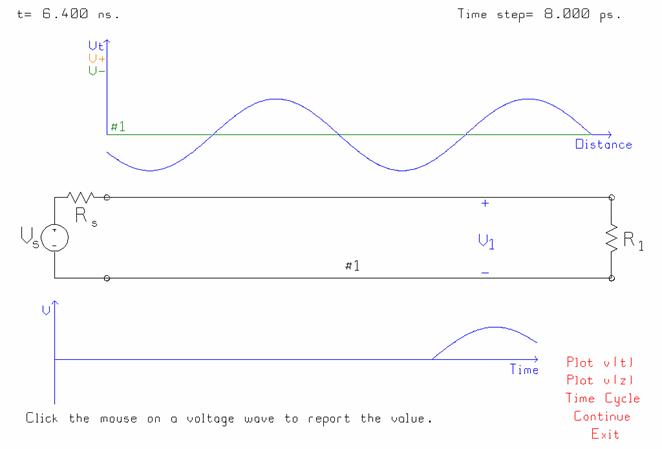
Fig. 45 A transmission line with a sinusoidal generator.
In Fig. 45, time has advanced to 6.4 ns, and the leading edge of the generator’s sine wave has almost reached the load. The voltage at the voltmeter V1, located at 150 cm from the generator, has about a half cycle of the incident sine wave. We expect the reflected sine wave to have amplitude 5x(25-50)/(25+50)=-1.667 volts. By decomposing the voltage on the transmission line into Vplus and Vminus, we can observer the incident wave, the reflected wave, and the transmitted wave simultaneously.
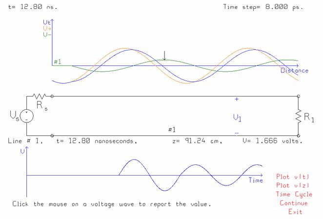
Fig. 46 The incident, reflected and total voltages on the transmission line.
Letting time advance to 12.8 ms is enough for the reflected wave to travel almost all the way back to the generator. The voltage-vs.-distance graph at the top of Fig. 46 show the incident or positive-going traveling wave in red, with a constant amplitude of 5 volts. The reflected or negative-going traveling wave is shown in green, and has amplitude 1.666 volts as expected. The blue curve is the total voltage, which is the sum of the incident and the reflected wave. At the bottom of Fig. 46 we see the voltage at the voltmeter location, half a wavelength from the load. After once cycle of the five-volt incident wave, the reflected wave reaches the voltmeter, and the amplitude changes to 5-1.666=3.334 volts.
11 Demonstrations Using BOUNCE
Program BOUNCE is used in class to demonstrate various wave phenomena[2]. A discussion of the demonstrations is available by clicking here: Basic Demonstrations with BOUNCE [3]. This document lets you fetch the "bnc" file for each simulation so that you can run it yourself and enjoy the animation.
12 Circuits Available in BOUNCE
The entry menu offers a choice of nine “circuit templates”, which are described in the following. In addition, expert users can create new circuits by editing the “bnc” file to add new branches and loads. Note that the loads terminating any of the transmission lines can be changed to parallel or series RL or RC circuits.
12.1 Simple Transmission Line
The first circuit template is the simplest, but is the most useful, and has been shown in Fig. 2. It consists of a voltage generator with an internal resistance, a transmission line of a given characteristic resistance and propagation velocity, and a load. This circuit is used with a step generator to demonstrate basic wave propagation, absorption by a matched load, reflection from an unmatched load, from a short circuit and from an open circuit. Use a pulse generator to demonstrate reflection of a pulse. Use an unmatched generator to demonstrate a pulse that reflects back and forth along the line between unmatched terminations.
This circuit template can be used to demonstrate a sinusoidal “traveling wave” being absorbed by a matched load. By changing the load to an open circuit or a short circuit, this circuit template can be used to demonstrate a traveling wave reflected back on itself. The wave then gradually changes to a standing wave. The concepts of “traveling wave” and “standing wave” are fundamental. With an unmatched load, such as a 25 ohm load terminating a 50 ohm line, partial reflection can be demonstrated, as was discussed above in Figs. 45 and 46. The wave is a combination of a standing wave and a traveling wave, and the circuit template can be used to show the concept of “standing wave ratio”.
12.2 Two Transmission Lines in Series
The circuit template having two transmission lines in series has been used in Figs. 39 to 44 to demonstrate simple reflection and transmission through a junction. The problem can be made more complicated and interesting if the generator and the load are both unmatched. Then there are reflections from the left and the right which travel back to the junction, leading to multiple interactions. Also, a sinusoidal generator can be used to demonstrate transmission onto an unmatched transmission line. If the load is matched to the right-hand line, there will be a standing wave on line #1 and a traveling wave on line #2.
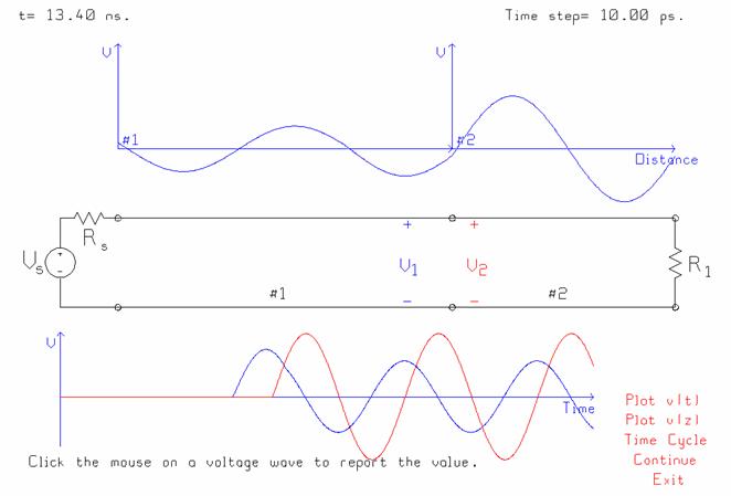
Fig. 47 Transmission of a sinusoid onto an umatched line. At 13.4 ns, the voltage on line #1 is quite small.
In Fig. 47, a 10 volt, 50 ohm sinusoidal generator at 300 MHz drives a 1.5 m, 50 ohm line in series with a 1 m, 100 ohm line, terminated in a 100 ohm resistor. The propagation speed is 30 cm/ns on both lines. The transmission coefficient is 1.333 so the transmitted sine wave has amplitude 6.667 volts, and is seen as the voltage at voltmeter #2, in red in Fig. 47. Voltmeter #1 shows the initial sine wave of amplitude 5 volts changing into the incident plus the reflected wave, of net amplitude 3.333 volts. The voltage as a function of time on line #1 is interesting because it varies from the small-amplitude sinusoid of Fig. 47 to the large-amplitude sinusoid of Fig. 48. This demonstrates the time variation of the voltage on a transmission line with a standing wave ratio of two.
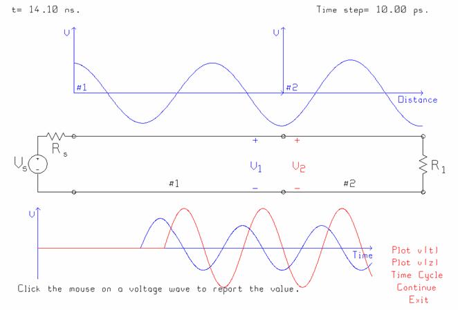
Fig. 48 At 14.1 ns, the voltage on line #1 is large.
12.3 Three Transmission Lines in Series
The third circuit template consists of three transmission lines in series, shown in Fig. 49. For example, a 50 ohm line might be connected to a 73 ohms line, thence to a 50 ohm line and a 50 ohm load. The “mismatched” line causes a wealth of reflections. The circuit can also be used to demonstrate the quarter-wave transformer, discussed below.
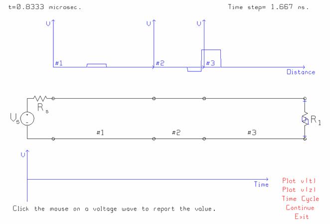
Fig. 49 The circuit template having three transmission lines in series.
In Fig. 49, the generator has amplitude 10 volts, internal resistance 50 ohms, and pulse width 0.1 microsec. Line #1 has length 100 m, characteristic resistance 50 ohms, and speed of propagation 20 cm/ns. Line #2 is 50 m in length, with 73 ohm characteristic resistance, and 20 cm/ns speed. Line #3 is 100 m long, with 50 ohm characteristic resistance, and 20 cm per ns speed, and is terminated with a matched load. Fig. 49 shows that at a time of 833.3 ns, there is a reflected pulse on line #1 of 0.935 volts amplitude, arising from the initial reflection at the junction of line #1 and line #2. The incident pulse has propagated as far as the junction between line #2 and line #3, and is being partially reflected and partially transmitted. The transmitted amplitude is 4.825 volts, and the reflected amplitude is -1.110 volts. As time advances, this -1.110 volt pulse will be re-reflected from the junction between line #1 and line #2.
12.4 Two Lines in Series with Shunt Load
The circuit template of Fig. 50 consists of two transmission lines with a shunt load. This circuit can be used to demonstrate the formulas for transmission and reflection for this interconnection.
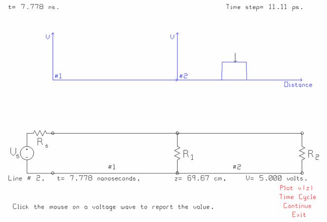
Fig 50 Two transmission lines in series with a shunt load.
In Fig. 50, the generator is a 1 volt pulse, 1 ns wide, and has internal resistance 25 ohms. It drives a 25 ohm line of length 1.5 m and wave speed 30 cm/ns, in series with a 1.5 m line of characteristic resistance 50 ohms and speed 30 cm/ns, which is terminated with a 50 ohm resistor. To obtain a match at the junction, a 50 ohm shunt resistor has been used. Fig. 50 shows that there is no reflection from the junction and that the pulse transmitted onto line #2 has amplitude 5 volts, as expected.
12.5 Two Transmission Lines in Series, with a Branching Transmission Line
Fig. 51 shows the circuit template for two transmission lines in series with a short branch. This circuit can be used to simulate a computer bus having a short branch to a high-resistance listener. In Fig. 51, the generator is a step function of 5 volts amplitude, and has an internal resistance of 100 ohms. The step’s rise time has been set to 0.1 ns. All three lines have speed of propagation 14 cm/ns and characteristic resistance 50 ohms. Line #1 is 3 cm long, and line #2, 9 cm. The branch is 2 cm in length. The transmission lines are terminated with 1 pF capacitors, representing the input capacitance of a CMOS gate. Multiple reflections back and forth on the branch lead to ringing at the voltage seen by an observer at the end of line #2.

Fig. 51 The circuit template for two transmission lines in series with a branch.
Let time advance until 0.8 ns to get the response shown in Fig. 51. The leading edge of the generator’s step is about to reach the load, C1. The rise time of the step of 0.1 ns is clearly seen as a linearly-increasing voltage from zero to 1.11 volts. This voltage represents the voltage divider at the source, multiplied by the transmission coefficient through the junction. Enough time has gone by that there have been multiple interactions on the short branch. The voltage wave has not yet reached the V1 voltmeter at the load, so the graph at the bottom in Fig. 51 shows zero volts.
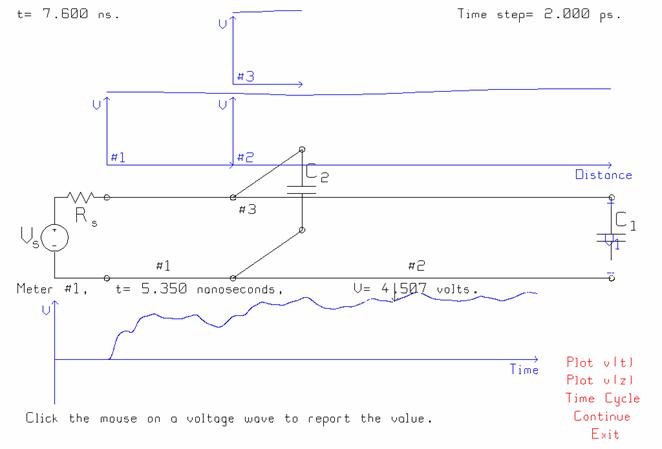
Fig. 52 The voltages at time=7.6 ns.
Allowing time to advance to 7.6 ns permits many trips back and forth on the lines, and many interactions at the junctions and loads. The voltage V1 at the load gradually increases with many peaks and valleys. A minimal “logical 1” voltage of 4.5 volts is attained at 4.888 ns, but the voltage subsequently falls to 4.473 volts at 5.286 ns, not sufficient for a logical 1. At 5.35 ns, the voltage rises above 4.5 volts and does not subsequently fall below, and this is the delay time associated with this circuit.
In an A.C. context, the two-lines-in-series-with-branch circuit template can be used to demonstrate single-stub matching, including the transient from the turn-on of the generator to the sinusoidal steady state. Initially the match is poor, but as steady state is built up, the match becomes perfect.
12.6 Transmission Line with Two Branching Points
Fig. 53 shows the circuit template having three transmission lines with two branches. In an A.C. context, this circuit template can be used to demonstrate double-stub matching, including the transient from the turn-on of the generator to the sinusoidal steady state. The component values for this circuit are built in to the program and are used when this circuit template is selected.
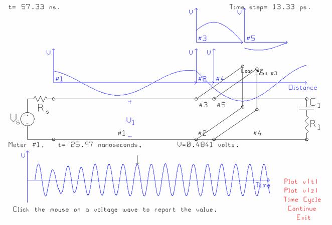
Fig. 53 The circuit template having a three transmission lines with two branches.
The circuit in Fig. 53 consists of a 1 volt amplitude, 50 ohm generator at 300 MHz. All five transmission lines have characteristic resistance 50 ohms, and speed of propagation 300 meters per microsecond. Line #1 is 1 m long, sufficiently long that we will be able to see if the voltage on the line is a “standing wave” or a “traveling wave”. Line #2 is 0.125 m or an eighth wavelength; line #4 to the load is 0.125 m. The stubs are terminated with short circuits. The load is 73 ohms in series with 12.93 pF. The lengths of the stubs can be designed with the aid of program TRLINE [5,6] to be 0.399 m for line #3 and 0.368 m for line #5, and then TRLINE reports the SWR on line #1 as 1.024, a reasonably good match. These values can be entered into BOUNCE. When BOUNCE is run, we see that the leading edge of the generator’s sinusoid is reflected from the first junction, so initially there is no match. It takes a few cycles of the sinusoid to build up the match. Fig. 53 shows the voltage in the middle of transmission line #1. Initially, there are a few cycles of non-constant amplitude, but by approximately the fifth cycle the double-stub circuit has reached the sinusoidal steady state. As time progresses the amplitude of the voltage wave on line #1 is nearly constant as it travels along the line, and so the load is matched.
It is instructive to change the frequency and verify that the match is poor at, for example, 150 or 600 MHz. TRLINE can calculate the bandwidth of the match.
The two-branch circuit can be used to simulate a computer bus with two branches to high-impedance “listeners” with capacitive inputs. Ringing on the branches causes the “rise time” and “fall time” at the load to be quite long.
12.7 Transmission Line with Three Branches
Fig. 53 shows the circuit template having three branches. In a logic-design context, this template can be used to study a bus loaded with three branches to listening devices. In an A.C. context, the circuit can model triple-stub matching, or a low-pass filter for the specific circuit in Fig. 53.
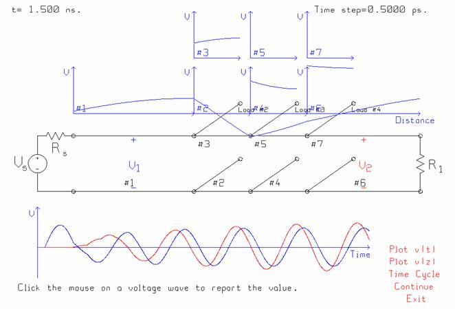
Fig. 53 The circuit template with three branches.
In Fig. 53 the generator has amplitude 1 volt and internal resistance 50 ohms. All the lines have propagation speed 300 meters per microsecond. The load is 50 ohms. The input line, #1, is 2 cm in length, and the output line, #6, is also 2 cm in length. Lines #2 and #4 are both 0.9375 cm long, with characteristic resistance 217.5 ohms. The stubs, lines 3,5, and 7, are all 0.9375 cm long. Lines 3 and 7 have characteristic resistance 64.9 ohms, and line 5, 70.3 ohms. This low-pass filter design is found in Pozar’s textbook [7]. The component values for the low-pass filter circuit are built in to the BOUNCE program and are used when this circuit template is selected.
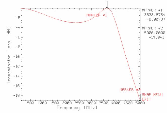
Fig. 54 The frequency response of the low-pass filter of Fig. 53.
The TRLINE program can be used to calculate the frequency response of the low-pass filter. At 3638 MHz, the transmission loss is nearly zero, and the filter passes the wave almost unattenuated. But at 5000 MHz, the transmission loss is about 19 dB. In Fig. 53, BOUNCE is used to find the transient response of the filter at 3638 MHz. There are a couple of cycles of transients in the V1 voltage on the input line, and then steady state settles in. Similarly, at V2 on the output line, after some initial transient behavior, the output voltage becomes approximately equal to that at the input. The TRLINE program reports that the SWR on the input transmission line is 1.01, so the filter absorbs most of the energy incident on it, and transmits it through to the output.

Fig. 55 The filter response at 5000 MHz.
Changing the frequency to 5000 MHz obtains the transient response shown in Fig. 55. The output voltage shows some initial transient behavior then settles to an amplitude of 0.0425 volts. There is a high standing-wave ratio on the input transmission line, reported by TRLINE as 319. The filter reflects most of the engery incident on it.
12.8 Quarter Wave Transformer
BOUNCE includes two more special cases of circuits for demonstration purposes, namely a quarter-wave transformer and a power splitter. A quarter-wave transformer is often used in microwave and RF circuits to obtain a match between dissimilar transmission lines. This circuit can be used to demonstrate the match that is obtained, and the transition from turning on the sinusoid to the sinusoidal steady state. Also, in the context of digital circuits, this circuit shows that the “match” provided by a quarter-wave transformer is not without value.
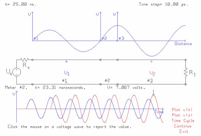
Fig. 56 The quarter-wave transformer circuit.
Fig. 56 shows the three-lines-in-series circuit template loaded with the quarter-wave transformer parameters. The generator is 1 volt amplitude, 50 ohm resistance, at 300 MHz. The three lines have wave speed 300 m per microsec. Lines 1 and 3 are 1 m long, and line 2, a quarter-wavelength at 300 MHz, or 25 cm. Line 1 has characteristic resistance 50 ohms, and line 3, 100 ohms, and the load resistor is 100 ohms. The transformer is designed to match 100 ohms to 50 ohms with a characteristic resistance of the square root of 100x50, or 70.711 ohms. Running BOUNCE shows that the match is obtained in about one cycle of the sine wave. Fig. 56 shows that at the design frequency the transformer passes the signal as expected. The input line is almost perfectly matched. The amplitude of the output voltage is 7.067 volts.
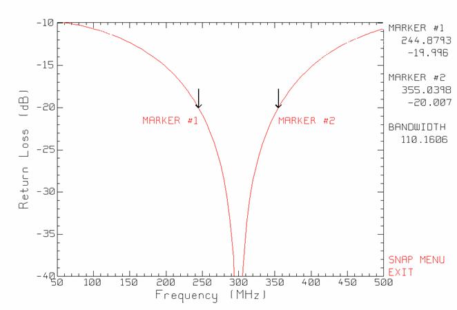
Fig. 57 The return loss of the quarter-wave transformer.
Fig. 57 was calculated with TRLINE [5,6] and shows the return loss of the quarter-wave transformer from 50 MHz to 500 MHz. The bandwidth for a return loss better than -20 dB extends from about 245 to about 355 MHz. A return loss of 20 dB corresponds to a reflection coefficient of 1/10, and a VSWR of 1.222. Change the frequency in BOUNCE to 355 MHz to see the time response of the transformer at the upper end of the 20 dB bandwidth.
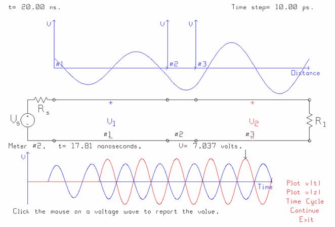
Fig. 58 The response of the quarter-wave transformer at 355 MHz.
Running BOUNCE at 355 MHz obtains the time response shown in Fig. 58. The output voltage is 7.037 volts, down a small amount from 7.067 volts at the center frequency. Watching the voltage on the input line as time progresses shows that the match at the input is imperfect. TRLINE reports the VSWR on the input line is 1.222, as expected. This value can be obtained from BOUNCE as well, by carefully finding the largest voltage on the input line and the smallest voltage on the input line, over one time cycle of the AC generator.
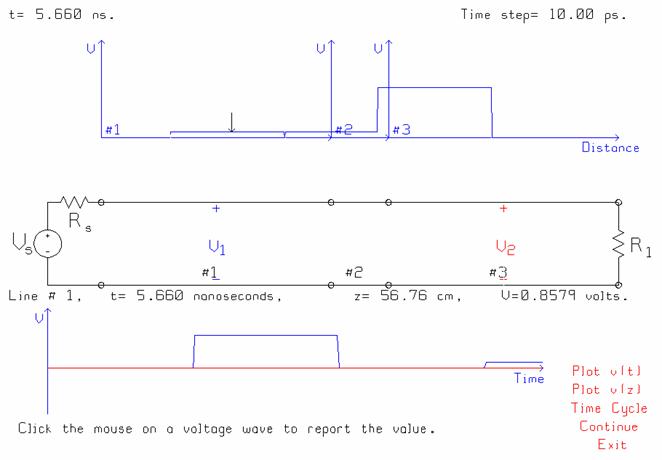
Fig. 59 The pulse response of the quarter-wave transformer.
What happens if a quarter-wave transformer is used to “match” a 50 ohm line to a 100 ohm line in a digital circuit? Consider a clock frequency of 300 MHz, leading to the “quarter-wave” length of the transformer of 12.5 cm in the circuit of Fig. 58. Take the pulse length as half a clock cycle, 1.667 ns. If the 50 ohm line is connected directly to the 100 ohm line, the reflection coefficient is 1/3 so the reflected pulse amplitude is 1.6667 volts. Fig. 59 shows the response of the quarter-wave transformer, at a time of 5.66 ns. The input of the transformer does not perfectly absorb the incident pulse; there is a reflected pulse of 0.8579 volts, which is better than the reflection if the transformer were not used. The energy trapped in the transformer bounces back and forth, releasing some additional small reflected pulses.
12.9 Power Splitter
The last circuit template offered by BOUNCE as a built-in circuit is the power splitter. The circuit template is shown in Fig. 60. It comprises three transmission lines in series, with a branch at the 2nd junction. The power supplied by the AC generator must be split between the two load resistors equally, with a match at the generator terminals at the center frequency.
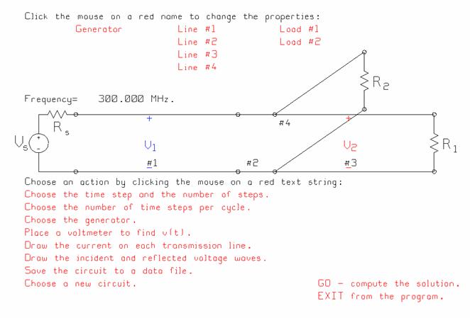
Fig. 60 The power splitter circuit template.
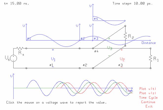
Fig. 61 The time response of the power splitter.
The power splitter consists of two 50 ohm lines branching from the same point, providing a 25 ohm net load. A quarter-wave transformer is used to match this 25 ohm parallel combination to the “input” 50 ohm line. All the lines have wave speed 30 meters per microsecond. The characteristic resistance of the transformer is the square root of 50 times 100, or 70.711 ohms. At the center frequency of the transformer, a perfect split of the incoming sinusoid into two equal parts is obtained. The two output voltages in Fig. 61 are equal, and the match on the input line is perfect.
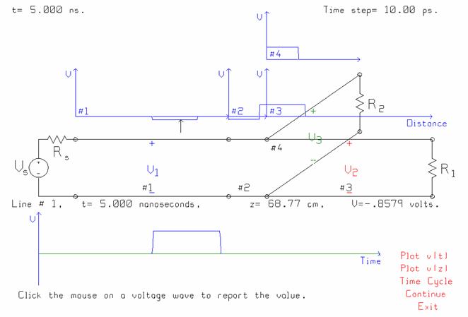
Fig. 62 The response of the power splitter to a 1 ns pulse.

Fig. 62 The response of the power splitter to a pulse input.
Fig. 62 shows the response of the power splitter to a 1 ns pulse at the input. The splitter still divides the input pulse equally between the two output “channels”. However, the match at the input is imperfect, so there is some reflection back to the generator.
13 Saving a Circuit as a “bnc” Data File
Often in using BOUNCE you will enter all the component values for a circuit, work on the response, and then you will want to save the component values to a file, so that when you return to the problem later, you will not have to re-enter them all over again. In the main menu of Fig. 2, click the mouse on “Save the circuit to a data file”. BOUNCE will ask for a file name. The standard extension is “bnc” for circuit files for the program. Typing F10 saves the file. When you exit from BOUNCE, the program writes a setup file called BOUNCE.SET, which remembers the name of your data file. When you re-start the program later, BOUNCE will fetch your data file and reload all the values for your circuit.
You can also tell the program to load a saved circuit explicitly. In the simulation menu of Fig. 3, click the mouse on “Choose a new circuit”. This gets the entry menu of Fig. 2, and you can click the mouse on “Read a saved circuit”. BOUNCE shows a menu asking for the “bnc” file name, and then loads the circuit.
Expert users can edit the “bnc” file to create new circuit templates not offered by BOUNCE itself.
14 Conclusion
BOUNCE is intended as a learning tool for students taking a first course in “electromagnetic fields and waves”. Reference [2] describes various demonstrations of wave phenomena using BOUNCE. The animation helps in visualizing how the waves travel on transmission line circuits and how they interact with junctions and loads. Ref. [2] also describes some demonstrations that are relevant for computer engineering students, to make them aware of the importance of matching considerations in digital circuits. Ref. [3] contains brief descriptions of some of the demonstrations done in the classroom with the BOUNCE program. BOUNCE is particularly useful for students as a “laboratory” to verify pencil-and-paper solutions to transmission line problems solved with a “bounce diagram” or “lattice diagram”.
15 References
[3] C.W. Trueman, Basic Demonstrations with BOUNCE, Electromagnetic Compatibility Laboratory, Concordia University, November 1, 2001.
[4] S.H. Russ, “Electromagnetic Effects in High-Speed Digital Systems”, Chapter 10 in J.D. Kraus and D.A. Fleisch, “Electromagnetics With Applications”, McGraw-Hill, 1999.
[5] C.W. Trueman, “Interactive Transmission Line Computer Program for Undergraduate Teaching”, IEEE Trans. On Education, Vol. 43, No. 1, February, 2000.
[6] C.W. Trueman, TRLINE User’s Guide, Electromagnetic Compatibility Laboratory, Concordia University, 2001.
[7] D.M. Pozar, “Microwave Engineering”, Addison-Wesley, 1990.
Dr. C.W. Trueman,
Professor,
Department of Electrical and Computer Engineering,
Concordia University.