User’s Guide for Program RLAPL
Scalar Potential in Resistors of Varying Geometry and Resistivity
C.W. Trueman
September 20, 2000.
Updated September 25, 2001.
Consider the problem of
finding the resistance of a resistor of uniform thickness t. The resistor has two metallic terminals, one
at potential ![]() volts and the other
grounded. The resistor can have any
arbitrary shape in the xy plane provided that its thickness is uniform. The resistivity of the material
volts and the other
grounded. The resistor can have any
arbitrary shape in the xy plane provided that its thickness is uniform. The resistivity of the material ![]() can vary throughout
the resistor. The problem is to find
the scalar potential
can vary throughout
the resistor. The problem is to find
the scalar potential ![]() in the resistor, and
hence the current flow at each point in the resistor,
in the resistor, and
hence the current flow at each point in the resistor, ![]() where
where ![]() . The current flow in
the resistor can then be found by integrating the current density over a
cross-sectional surface in the resistor.
. The current flow in
the resistor can then be found by integrating the current density over a
cross-sectional surface in the resistor.
This User’s Guide presents a
finite-difference method for finding the scalar potential and hence the current
flow in the resistor. The method is
implemented in a program called RLAPL.
First the update equation for the finite-difference method will be
derived, and then the input commands for the RLAPL program are given. Some simple examples are then solved.
Students wishing to use
program RLAPL should read the user’s guide for program LAPL, which solves
Laplace’s Equation in regions of space filled with dielectric, such as coaxial
cable. The LAPL user’s guide provides background needed to understand the
following. To get a copy of the “exe”
file for the program, click the mouse here:
Get rlapl.exe.
The Partial Differential Equation for the Scalar Potential
This sections obtains a
partial differential equation(PDE) that the scalar potential ![]() satisfies in the
resistor. Since there is no stored
charge in the resistor,
satisfies in the
resistor. Since there is no stored
charge in the resistor, ![]() . Since
. Since ![]() and
and ![]() we can carry out some
substitutions to derive the PDE, as follows.
we can carry out some
substitutions to derive the PDE, as follows.
Starting with
![]()
substitute ![]() where
where ![]() , and
, and ![]() to obtain
to obtain
![]()
A resistor of uniform thickness t is a two-dimensional problem
in which the scalar potential ![]() is a function of
is a function of ![]() and
and ![]() only. Expanding the divergence and gradient in
rectangular coordinates obtains
only. Expanding the divergence and gradient in
rectangular coordinates obtains
![]()
hence
![]()
Note that if the conductivity ![]() is uniform, that is,
not a function of
is uniform, that is,
not a function of ![]() or
or ![]() , then this equation reduces to Laplace’s Equation. Hence Laplace’s Equation is the special case
of uniform conductivity.
, then this equation reduces to Laplace’s Equation. Hence Laplace’s Equation is the special case
of uniform conductivity.
The Update Equation for the Finite Difference Method
Consider a finite difference
solution of the PDE in a cell space of cell size ![]() having cells numbered
having cells numbered
![]() in the x
direction and
in the x
direction and ![]() in the y
direction. The centers of the cells
will be denoted by points
in the y
direction. The centers of the cells
will be denoted by points ![]() and the scalar
potential at the center of cell i,j is
and the scalar
potential at the center of cell i,j is ![]() .
.
To derive an update equation
for a finite-difference method, we need to approximate the partial derivatives
with the central difference formula. Let point “b” be half way between ![]() and
and ![]() and point “a” be half
way between
and point “a” be half
way between ![]() and . Then
and . Then
The partial derivatives at “a” and “b” are approximated as
![]()
and
![]()
To approximate the conductivity ![]() at “b” we can
consider current flowing from
at “b” we can
consider current flowing from ![]() to
to ![]() . For half the
distance the resistivity is
. For half the
distance the resistivity is ![]() and for half the
distance the resistivity
and for half the
distance the resistivity ![]() , so we have two resistors in series, each of length
, so we have two resistors in series, each of length ![]() . The resistance is
. The resistance is
![]()
where t is the thickness of the resistor. This can be written as
hence the equivalent resistivity for current flow from ![]() to
to ![]() is the average,
is the average,
![]()
where the “r” superscript stands for “right” and denotes the average
resistivity at the cell wall to the right of node i,j, which is point ![]() . Define the “right”
conductivity as
. Define the “right”
conductivity as
![]()
From above,

hence can now write the complete approximation to the first term in the
PDE as
![]()
Similarly if we define the
“top” conductivity as
![]()
then we can approximate the
2nd term in the PDE in a similar way. Inserting the approximations into the PDE and rearranging
obtains the update equation,
![]()
where
![]()
The “right”, “top” and
“tilde” conductivities can be computed as part of the initialization of the
program and stored in an array, and recalled when the update equation is
applied to cell ![]() .
.
Program RLAPL
Program RLAPL implements the method described above. To learn to use RLAPL, read the “LAPL User’s Guide” for the Laplace’s Equation solver called “LAPL”. RLAPL and LAPL are set up the same way and many of the LAPL commands will do the same thing in RLAPL. The following briefly describes the commands that are new in RLAPL and then gives some examples of calculations that can be done with RLAPL.
Table 1 lists the input commands
for program RLAPL and Table 2 is an input file which models a simple
resistor. The user should include
comments in the input file describing the purpose of each line in the file,
using the CM command. The cell size is
set with SIZE, in meters. The size of
the space is set with SPACE. By
definition all the edge cells in the space are metallic cells and are set to
zero potential. Some of these cells can
be reset to 100 volts or some other potential, but these cells cannot be
resistive cells or insulators. The
thickness of the resistor is set with THICKNESS, in meters. All the cells in the cell space, except the
metallic edge cells, start out as insulators, with a very high resistivity. A line of cells can be set to a desired
resistivity, say 10 ohm-m, with the RESIS_LINE command. All the cells inside a rectangular box can
be set a desired resistivity with the RESIS_BOX command. We can define metallic terminals for our resistor,
set to fixed potentials, with LINE, CIRCLE, CSHELL and ELLIPSE, as in program
LAPL. To find the resistance we set
one terminal of the resistor to a fixed potential such as 100 volts and the
other terminal to zero volts. Then we need to know the current flow I in the
resistor, so we can evaluate ![]() ohms. Use the command CURRENT to draw a line
across the resistor, either vertically or horizontally. The program will calculate and report the
current flowing across this line. Thus
in Table 2 the user asks for the current across a line at cell 10 axially, cutting
across the full width of the resistor from cell 1 to cell 54.
ohms. Use the command CURRENT to draw a line
across the resistor, either vertically or horizontally. The program will calculate and report the
current flowing across this line. Thus
in Table 2 the user asks for the current across a line at cell 10 axially, cutting
across the full width of the resistor from cell 1 to cell 54.
The commands for controlling iteration in RLAPL are the same as those in program LAPL. Usually a large number of iterations such as 20,000 is required, and it is convenient to have the program update the graphics display every 1000 iterations so that you can monitor the progress of the computation.
Program RLAPL creates two “table” files for graphing with CPLOT. The scalar potential is saved in VOLTS.TBL and the magnitude of the electric field vector is saved in EFIELD.TBL. Note that the value of the current is written into the header in VOLTS.TBL, in case you forget to note it when it appears on the computer screen.
Table 1
Input Commands for Program RLAPL
|
Purpose |
Command |
|
Include a descriptive comment in the input file |
CM followed by your text |
|
Specify the cell size (meters) |
SIZE 0.01 |
|
Specify the size of the finite-difference cell space |
SPACE 10 12 |
|
Define the thickness of the resistor |
THICKNESS 0.001 |
|
Set the resistivity of a line of cells to 10 ohm-meters |
RESIS_LINE 2 3 45 52 10. |
|
Set the resistivity of a box of cells to 10 ohm-meters |
RESIS_BOX 2 3 101 52 10. |
|
Define a line of cells as an insulator |
INSUL 2 2 101 2 |
|
Define a line of cells at a fixed potential |
LINE 10 10 20 10 0. LINE 10 10 10 20 100. |
|
Define a solid cylinder of cells at a fixed potential |
CIRCLE 50 50 10 100. |
|
Define a hollow cylindrical shell of cells at a fixed potential |
CSHELL 50 50 40 0. |
|
Define a hollow elliptical shell of cells at a fixed potential |
ELLIPSE 50 50 60 30 0. |
|
Find the current flowing across a line |
CURRENT 10 1 10 54 |
|
Specify the total number of iterations to be done |
NSTOP 10 |
|
Pause the program after updating each cell |
SINGLESTEP |
|
Redraw the potentials after 10 iterations of updating the cell space |
NUPDATE 10 |
|
Pause the program after redrawing the potentials |
PAUSE |
|
Mark the end of the input file |
END |
Simple Resistor
Find the resistance of a resistor of thickness 1 mm, resistivity 10 ohm-m, measuring 1 cm long and 0.5 cm wide.
Answer: ![]() ohms
ohms
To model this with RLAPL,
choose a cell size of 1 cm / 100 cells = 0.01 cm = 0.0001 m. The resistor is 100 cells long by 50 cells
wide. Table 1 gives the input file. The input for program RLAPL is quite
similar to that for program LAPL, and users should read the “LAPL User’s
Guide”. In Table 2, SIZE sets the cell size to 0.0001 m. The thickness of the resistive material is
set to 1 mm with THICKNESS. The size
of the cell space is set to 102 by 54 cells.
Lengthwise, 102 cells is made up of 1 cell for the 100-volt metallic
contact at left, 100 cells for the 1 cm body of the resistor, and 1 cell for
the grounded metallic contact at the right.
Crosswise, 54 cells is made up of 1 cell for the metal boundary of the
cell space, 1 cell for an insulator to
separate the body of the resistor from the metal boundary, 50 cells for the
half centimeter width of the resistor, plus one cell for an insulator and 1
cell for the metal boundary. The resistivity
of the body of the resistor is set up with the “RESIS_BOX” command, which sets
all the cells inside the rectangle from cell 2,3 to cell 101,52 to 10
ohm-meters resistivity. Note that we do
not set the cells from 2,2 to 101,2 or from 2,53 to 101,53 to be
resistive. These cells are the
insulator separating the resistor from the metal boundary of the cell
space. Next the 100 volt terminal of
the resistor is set up with a LINE of cells at 100 volts from cell 1,3 to cell
1,52. The 0 volt terminal is set up
with a LINE of 0-volt cells from 102,3 to 102,52. Because the edge cells are already at 0 volts by default this
could be omitted. The insulators
separating the body of the resistor from the metal wall at the bottom and at
the top are explicitly defined with “INSUL” commands. These set up a line of insulating cells from 2,2 to 101,2 and
from 2,52 to 101,53. Since the cells
are insulating by default, these commands could also be omitted. Including these commands makes the user’s
intentions clear and someone else reading the file will understand that these
cells are specifically intended to be insulating cells. The input file finishes by specifying 20,000
iterations be done and that the graphics screen be updated every 1000
iterations.
Table 2
Input file for
program RLAPL to model a simple resistor.
|
CM
Simple resistor for solution with RLAPL CM
CM
Resistor 1 cm long by 1/2 cm wide. CM
Thickness 0.1 cm CM
Resistivity 10 ohm-meter CM CM
CELLSIZE (in meters) is 100 cells= 1 cm or .01/100 = 0.0001 SIZE 0.0001 CM
The thickness of the resistive material: THICKNESS 0.001 CM CM
The resistor body will be 100 by 50 cells. CM
In addition, there is a 1 cell boundary all around the edges, CM
which is by definition a metal. We
need an insulator 1 cell CM
wide along the sides, to separate the resistor body from the CM
metal wall. This makes the width of
the cell space 4 more cells CM
than 50 cells=1/2 cm. SPACE
102 54 CM CM
Define the resistivity of cells in the body of the resistor CM
This fills a box 100 cells long and 50 cells wide, from cell 2,3 CM
to cell 101,52, with material of resistivity 10 ohm-meters. RESIS_BOX
2 3 101 52 10. CM CM
Define the metal contacts on the ends of the resistor. CM
The left edge where the current enters is at 100 volts: LINE
1 3 1 52 100. CM
The right edge where the current leaves is at 0 volts: LINE
102 3 102 52 0. CM
Note that all other boundary cells are grounded by definition, CM
so this last "LINE" command is not really needed. CM CM
Define the insulating boundaries along the sides. These cannot include CM
any edge cells: INSUL
2 2 101 2 INSUL
2 53 101 53 CM
Note that these “INSUL” commands are not really needed, either, CM
because all the cells in the cell space start out as "insulator"
cells CM
by default. CM CM
Find the current flowing across a vertical line centered at CM
cell I=10 cutting across the full width of the cell space from CURRENT 10 1
10 54 CM CM
Number of iteration between screen updates: NUPDATE 1000 CM
Total number of iterations: NSTOP 20000 CM END |
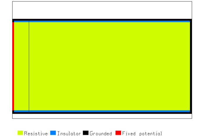
Figure 1 A simple resistor
consisting of insulating walls at bottom and top, and a uniform resistive body.
Fig. 1 shows the geometry created by the input file of Table 2. The edge cells of the space are all grounded metallic cells, shown in black, except the left-hand terminal of the resistor, which is shown in red to represent metallic cells at 100 volts potential. The resistive material is shown in yellow. The resistor body is separated from the metal wall at the top and bottom by insulating cells shown in blue. The black line running across the resistor at left is the cut specified by the CURRENT command in Table 2, at cell 10. The program will find the current flowing across this line.
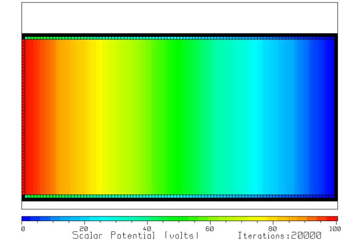
Figure 2 The scalar
potential in the resistor after 20,000 iterations.
Figure 2 shows the scalar potential that the program calculates in the simple resistor. The fixed potential cells at left are outlined in black. The row of insulating cells at the top and bottom of the resistor are also outlined in black to distinguish them from the resistive cells making up the resistor. The scalar potential decreases linearly from 100 volts at left (red) to zero volts at right (blue), progressing through the color scale representing the various voltage levels, yellow for 75 volts, green for 50 volts, cyan for 25 volts and so forth. If you run this problem with RLAPL you will note that the solution does not much change after about 10000 iterations, so the total of 20000 used here is larger than really needed.
The program reports that the current flowing across the line in Fig. 1 is 0.005005388 amps. Since the voltage was set at 100 volts, the resistance is
![]() ohms
ohms
Compared to the true value
of 20,000 ohms, the error is 0.11 percent.
Series Resistors
If we make cells 2 to 50 have resistivity 50 ohm-meters and cells 51 to 101 150 ohm meters. Then we have two resistors in series, each ½ cm long, and we expect the resistance to be 50000 ohms for the first half and 150000 ohms for the second half for a total of 200000 ohms. For 100 volts applied to the resistor, there should be a voltage drop of 25 volts over the 50000 ohm resistor and 75 volts over the 150000 ohm resistor. We can change the input file of Table 2 to define the series resistors with
RESIS_BOX
2 3 51 52 50.
RESIS_BOX
52 3 101 52 150.
The first RESIS_BOX command sets cells 2 to 51 from left to right to 50 ohm-meters and the second RESIS_BOX command sets cells 52 to 101 to 150 ohm-m. Then we run RPLAL to compute the solution.
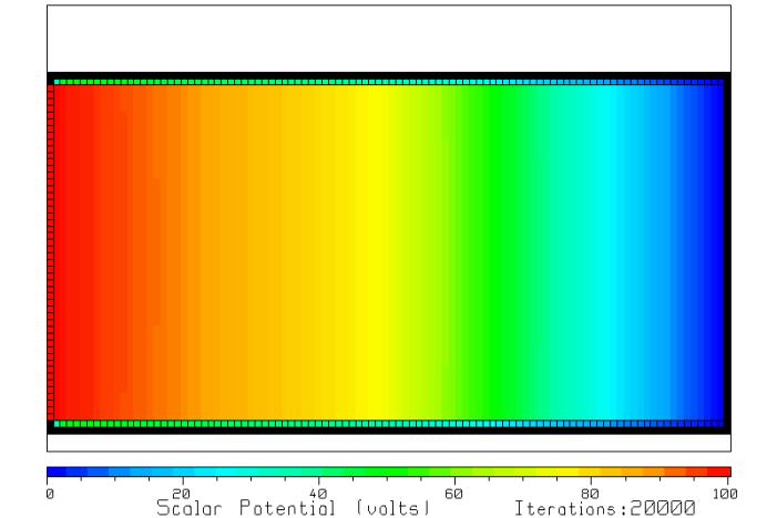
Figure 3 The
scalar potential for series resistors.
Figure 3 shows a
voltage drop from 100volts(red) at left to 75 volts(yellow) in the center of
the resistor, or 25 volts over the low-resistance half. Then the voltage drops from 75 volts in the
center to 0 volts at right over the high-resistance half. The program reports the current flow as
0.000508358 amps, so the resistance is 196,711 ohms, close to the value of
200000 ohms that is expected.
Parallel Resistors
Consider two
resistors side by side each 1 cm long and ¼ cm wide. One has resistivity 50 ohm-m and the other 10 ohm-m. The resistances of 200000 ohms and 40000
ohms are in parallel for a net resistance of 33,333 ohms. To model parallel resistors, make cells 2 to
27 cross-wise have a resistivity of 10 ohm-m,
RESIS_BOX
2 3 101 27 10.
And
cells 28 to 52 have a resistivity of 50 ohm-m,
RESIS_BOX
2 28 101 52 50.
Run RLAPL.
The program reports a current flow of 0.003005329 amps, so the
resistance is 33,274 ohms, close to the expected value.
Bent Resistor
Consider a resistor constructed in an “L” shape. The long leg is 1 cm long, 1/4 cm wide, and has resistivity 10 ohm-m. The short leg is ½ cm long, ¼ cm wide and has the same resistivity. What is the resistance? The centerline path in this resistor is 1.25 cm long, so we can reasonably expect a resistance of about 50000 ohms. But the problem is difficult to solve analytically, and the finite-difference method offers a much more accurate estimate of the resistance.
We can define
this resistor with a cell space of 103 by 54 cells, as follows:
SPACE
103 54
RESIS_BOX 2 28 101 52
10.
RESIS_BOX
77 2 101 27 10.
LINE
1 28 1 52 100.
LINE 2 26 75 26 0.
LINE
75 2 75 25 0.
CURRENT 10 1
10 54
Figure 4 shows the resistor
that results from this definition. The
long leg of the “L” is located across the top and the short leg at right. A LINE command sets the left-hand contact of
the resistor to 100 volts. LINE
commands have been used to set up metal walls along the bottom edge of the
resistor from cell 2,26 to cell 75,26, and along the left edge of the short
leg, from cell 75,2 to cell 75,25.
These metal walls isolate the rectangle at lower left from the rest of
the problem, and the potential in this rectangle will always be zero
volts. Note that the metal walls are
separated from the resistor by an insulator 1 cell wide. The “CURRENT” command asks for the current
crossing the black line shown at left in the figure.
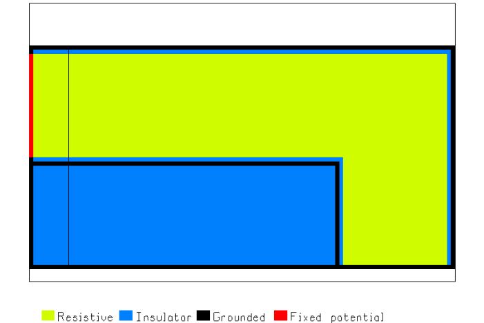
Figure 4 The
L-bend resistor.
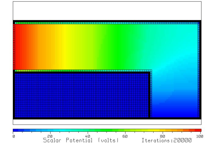
Figure 5 The
scalar potential in the L bend resistor.
Figure 5 shows the scalar potential in the L bend resistor after 20000 iterations. As might be expected, the potential varies roughly linearly with distance from the 100 volt contact at upper left to the 0 volt contact at lower right. The distortion in the equipotentials near the bend is of interest. This is more easily seen by graphing the file VOLTS.TBL with CPLOT, as in Figure 6.
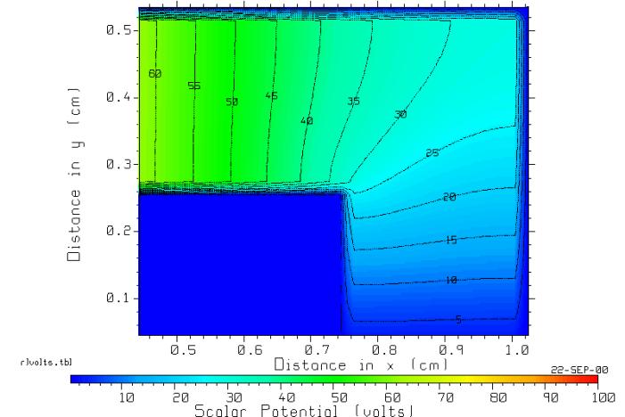
Figure 6 The equipotentials near the bend in the bent
resistor.
Fig. 6 shows the
equipotentials in the region of the bend, graphed with CPLOT. The 60 volt equipotentials at left is nearly
perpendicular to the edge of the resistor, as is the 5 volt equipotentials at
the lower right. The equipotentials
near the bend become distorted in shape.
The direction of current flow is perpendicular to the equipotentials,
and the current is largest where the equipotentials are close together. Thus, the current is largest near the inside
corner of the bend.
The RLAPL program
reports that the current flow in the resistor is 0.002181716 amps so the
resistance is 45,835 ohms, which is comparable to the expected value of about
50,000 ohms. The resistance is less
than the mean-path estimate because the current tends to “cut the corner” and
so the path length is effectively shorter than the mean path.
Resistor of Increasing Width
Suppose we have a resistor which is
t=1 mm thick and of resistivity ![]() 10 ohm-m. The
resistor is L=2 cm long, and increases in width from
10 ohm-m. The
resistor is L=2 cm long, and increases in width from ![]() ¼ cm at left to
¼ cm at left to ![]() ½ cm at right. What
is the resistance? The resistance can
be calculated by assuming the resistor is made up of a series connection of
resistors of length dx, and summing up their values to obtain
½ cm at right. What
is the resistance? The resistance can
be calculated by assuming the resistor is made up of a series connection of
resistors of length dx, and summing up their values to obtain
![]() ohms
ohms
This formula is, however, approximate, because it assumes that the current flow in the resistor is parallel to the bottom edge, and that the equipotentials are perpendicular to the bottom edge.
To model this resistor with RLAPL, set the space size to 202 by 54 cells of size 0.0001 mm, Then the resistor is 200 cells long, and should increase in width from 25 to 50 cells. The following commands define the resistor:
CM
Define the resistivity of cells in the body of the resistor
RESIS_BOX
2 3 201 53 10.
CM
Put a line of insulating cells to define the boundary of
CM
the resistor
INSUL
2 28 201 53
CM
Put a line of metal cells to make the field zero in the unused part
CM
of the cell space:
LINE 2 29 201 54
0.
CM
Define the metal contacts on the ends of the resistor
CM
The left edge where the current enters is at 100 volts:
LINE
1 3 1 27 100.
CM
Ask the program to find the current flowing in the resistor:
CURRENT
10 1 10 54
First we use RESIS_BOX to
fill the cell space with resistive material.
Then we define a line of insulating cells from cell 2,28 to cell 201,53
which is the sloped boundary of the resistor.
The resistor is then 200 cells long, and 25 cells wide at the narrow
end, increasing to 50 cells at the wide end.
We put a line of metal cells at zero potential adjacent to the
insulator, from cell 2,29 to cell 201,54.
This keeps the field zero in the upper left corner of the cell space. We set the voltage at the left hand side of
the resistor to 100 volts, and ask for the current crossing a vertical line at
cell 10. Figure 7 shows the geometry of
the resistor.
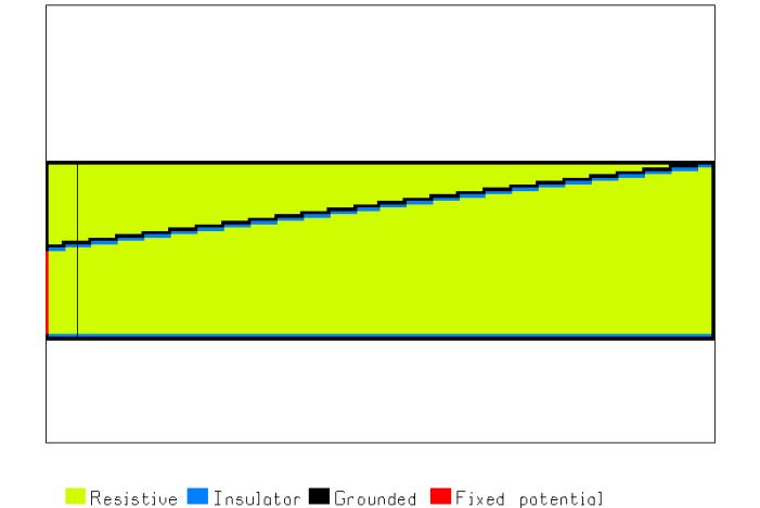
Figure 7 The resistor of
increasing width.
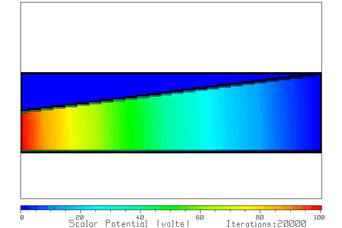
Figure 8 The
scalar potential after 20000 iterations.
Run program RLAPL and let it complete 20,000 iterations. The scalar potential is that shown in Fig. 8. The equipotentials are not perpendicular to the bottom edge of the resistor, but rather are curved as shown in Figure 9.
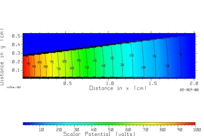
Figure 9 The equipotentials drawn with program CPLOT.
The equipotentials in Fig. 9 are not straight lines perpendicular to the bottom edge of the resistor, as assumed in deriving the formula given for the resistance, above. Hence we expect the value given by the formula will not be exact. The RLAPL program reports the current flow as 0.002002697 amps so the resistance is 49,932 ohms. This is about 10 percent low than the value of 55,452 ohms quoted above.
Notched Resistor
Consider a uniform resistor of length 1 cm, width ½ cm, thickness 1 mm, and resistivity 10 ohm-m. We showed above that the resistance is 20000 ohm. This was modeled with cells of size 0.0001 cm, so that the resistor is 100 cells long and 50 cells wide.
To trim the value of the resistance, a laser beam will be used to make two cuts in the resistive material, of width 0.0001 cm. The cuts are made near the center of the resistor and are of equal length. This forces the current to flow through the gap between the cuts, and increases the resistance. By controlling the width of the gap, the resistance can be controlled. Let us use program RLAPL to find the resistance for a gap width of say 1 mm.
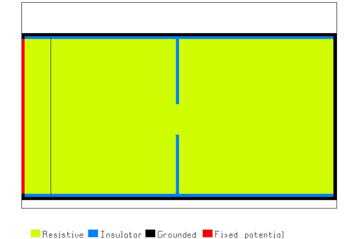
Figure 10 The uniform resistor with notches cut at each side.
Fig. 10 shows the resistor with notches cut at from the edge. The current must flow through the gap between the notches. By controlling the width of the gap, we can control the resistance.
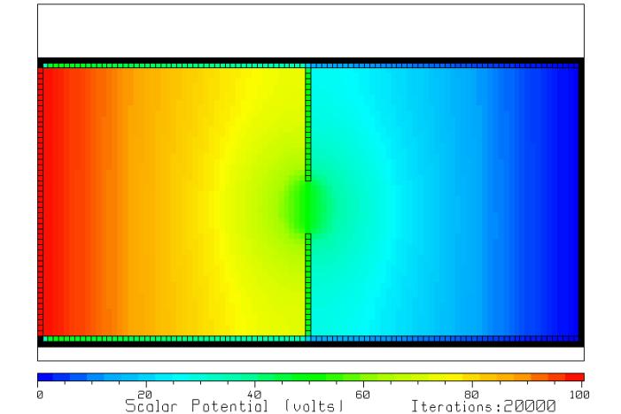
Fig. 11 The scalar potential after 20000 iterations.
Fig. 11 shows the scalar potential after 20000 iterations. Note that the colors at left and at right are not perfectly uniform from top to bottom; the solution may require more than 20000 iterations to converge. Try running it for more iterations. The potential drops from 100 volts (red) at left to about 70 volts (yellow) near the gap, then drops rapidly to 30 volts (cyan) on the other side of the gap, then declines gradually to 0 volts (blue) at right. A graph of the potential with equipotentials lines can be made with CPLOT, see Fig. 12.
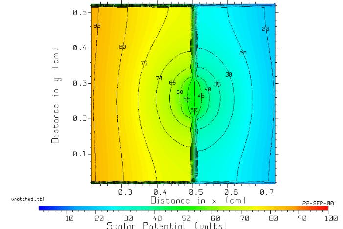
Fig. 12 The equipotentials in the region of the gap.
Fig. 12 shows the
potential in the center of the gap is 50 volts, which we expect from the
symmetry of the problem. The
equipotentials are roughly elliptical in shape surrounding the gap.
The RLAPL program reports the current as 0.003474683 amps, so the resistance with a 1 mm gap is 28,780 ohms, considerably higher than the value of 20000 ohms with no cuts in the resistor.
Conclusion