1 Introduction
Typical applications in
Evolutionary Computation often involve a direct and simple relation between
genotype and phenotype; Commonly, values from the genome are simply slotted
into a fitness function in a bijective mapping. While this approach is
sufficient for most practitioners, the dimensionality of the solution space
(phenotypes) is directly translated into the dimensionality of the space of
genotypes, potentially exceeding the size of space capable of being searched
by a Genetic Algorithm. For larger and more complex problems direct relations
between genotype and phenotype may be insufficient.
In a field inspired by Biology, it
is often useful to re-examine the source: the human genome may be viewed as a
tremendous compression of phenotypic complexity; The approximately 3 billion
chemical base pairs of the genome map to approximately 100 trillion cells [8].
It is clear that the process of development plays a significant role in the
addition of information to the phenotype; Indeed, models of biology often
attempt to re-create the hierarchical structure inherently formed by the
differentiation process, as in [5].
An emerging trend in
Evolutionary Computation is to create a (relatively) small and simple
genotype, and to increase the complexity of the phenotype through a
developmental process. The field of Artificial Morphogenesis spans a wide
array of approaches, varying on a gradient between total information being
contained in the genotype, to a bare minimum, where the genotype is a program
designed to spawn the phenotype. Some approaches use simple techniques, such
as the use of repeated structure when interpreting the genome. Another more
complex approach is the use of Grammars to develop agents, where the grammar
and initial conditions form the genotype. Such systems have enjoyed much
success, as in [11], where they were used in a theoretical experiment to study
the development of modular forms, or in [7], who used the model to develop a
neural network controlling a foveating retina. However, these systems are far
separated from their original biological metaphors.
Other equally complex
examples include developmental models, inspired by Embryogenesis. Examples
which attempt to model actual biological embryogenesis have also enjoyed much
success, as in the case of the particularly successful modeling of the
embryogenesis of a drosophilae, as found in [6]. In between direct models of
biology and models which are entirely divorced, there exists a class of
developmental models which seeks to abstract the developmental process to
high-level systems capable of artificial evolution, hopefully retaining some
of the high-level features of biological development. Bentley and Kumar [1],
and Eggenberger [3] both propose highly-simplified models which are used to
demonstrate the development of geometric and aesthetic principles. As is noted
in a review by Stanley and Miikulainen, simpler solutions may outperform
biologically plausible ones, and a need exists for abstraction [14]. Perhaps
most closely related to the subject of this paper, however, is work undertaken
by Dellaert and Beer [2]; This experiment aimed at the creation of a
computationally-tractable but biologically-defensible model of development,
aimed towards the evolution of agents capable of a locomotive task. Dellaert
and Beer's model consists of a conglomerate of cellular material, which
performed a series of differentiations. Differentiations begin as a single
symmetry-breaking division, followed by divisions controlled by a series of
Genetic Regulatory Networks. Drawbacks to this model resulted chiefly from the
size of the search space associated with their system. For example, they were
unable to evolve fit agents from scratch and hence began their experiments
with a hand-coded agent, from there obtaining results. Following this, their
model was simplified, using Random Boolean Networks ([9]).
This viewpoint, that of
increasing the complexity of the phenotype through the developmental process,
forms an interesting starting point for another emerging line of thought: It
has been postulated (most notably by Wolfram [15]) that natural selection
serves not to increase the complexity of agents through time, but instead to
limit the complexity inherent in a complex and unwieldy developmental process.
If this suspicion is correct, then the current typical use of Evolutionary
Computation may not utilize the metaphor of natural selection to its fullest
potential.
Wolfram suggests the use of
Cellular Automata as a model for the developmental process; The problem with
this approach is that the space of all CAs is notoriously large and difficult
to search. Attempts to evolve Cellular Automata to perform tasks may be found
in a review by Mitchell et al [12], where CAs were evolved to solve problems
of density classification and synchronization. While some of the burden was
alleviated through the use of stochastic approximations, searching through the
space of CAs proves to be tremendously computationally expensive.
In this paper, we present the
Bluenome
model of development. Bluenome is a highly abstracted model for developing
application-neutral agents composed of an arbitrarily large network of
components chosen from a finite set of types. Bluenome uses a subset of the
space of two-dimensional CAs, evolved in a genetic algorithm, starting from a
single neutral cell. In Phase One, Bluenome is applied to a series of
application-neutral experiments, designed to show that the system is capable
of producing interesting agents in a reasonable amount of time. In Phase Two,
it is applied to the problem of generating agents for an artificial but
non-trivial problem, contrasted against a bijective technique. It is our hope
to demonstrate that the Bluenome technique is a viable option for the design
of high-dimensional agents, by utilizing the features of the developmental
process, while abstracting enough so as to make evolution feasible.
2 The Bluenome Model
The Bluenome Developmental Model is a
highly simplified version of biological embryogenesis. It involves the
inclusion of a single component (Cell) into an array of spaces (Grid Cells),
and a methodology for that cell to grow into an agent, utilizing only local
information. The Cell contains a single piece of DNA, which it interprets to
decide its next action - the complexity of a piece of DNA is governed by
a system parameter, numRules, which limits its precision. The number of
possible cells is governed by a system parameter, numColours, the number
of types of components which might be included in an agent. This process is
limited by a system parameter numTel (number of telomeres) which acts as
a counter in each cell, decrementing with each action that a cell undertakes.
. An agent's
genome is comprised of a series of numRules rules, numRules
Î
N+. Each rule is
(numColours+2) integers long, leading to a total genome length of (numColours+2)*numRules.
Each rule is structured as:
|
colour
|
hormone1
|
.
|
hormonenumColours
|
action
|
where colour
Î
[1,numColours], hormonei
Î
[1,12], and action
Î
[1,numColours+3].
Initially, an agent
begins as a single neutral cell,
centred in an
environment (a square matrix of Grid Cells). When activated, a cell (currCell)
in the environment will collect hormones from its twelve
neighbourhood,
storing the number of occurrences of each cell colour in a list. The exception
is in the case of cells on the periphery; These cells are only included in the
count if the cells in between are empty
- hence the cell on the far, far left will be included in the count
only if the cell on the left is empty. What results is a list of numbers of
length numColours, each of value between zero and twelve.
Once any particular cell has collected
information regarding its neighbours, it searches the genome to find the
closest matching rule: First, it collects all rules in the genome such that the
current colour of the cell and the first argument in the rule match (If no such
rule is found, the cell takes no further action this time step). Next, it
searches that collection of rules for the one most closely matching its list of
current hormone levels (Euclidean distance). Finally, the action is extracted
from that rule. The action is executed by first decrementing the cell's
internal telomere counter (hence a cell may execute only numTel actions),
then executing the action corresponding to theRuleaction. Possible
actions include: Die, where a cell is removed, leaving an empty
Grid Cell; Specialize(colour), where a cell changes its colour to colour;
Divide, where a copy of the cell is placed in the best free
location; and Move, where the cell is relocated to the best free
location (if there are no free locations, no action is taken). It should be
noted that the best free location is defined as the Grid Cell in currCell's
four-neighbourhood furthest away from the largest mass of cells in the
eight-neighbourhood. In the case of equal distribution, the best free location
includes a directional bias - left, then counter-clockwise.
In this manner, a "good" genome will
allow a single initial cell to grow to a robust agent. The process terminates
when all telomeres are expended, or when there is no change from one
developmental time step to the next. No other mechanisms are included - there
are no special parameters for symmetry breaking, beyond that inherent in the
directional bias.
One view of this
process is as a subset of all 2-dimentional Cellular Automata with radius 3.
The key differences between CAs and Bluenome are: (1) Bluenome begins with a
single cell in the centre of a finite grid. Empty (white) cells cannot change
their colour without a non-white neighbour;
(2) As the hormone collection process does not note direction, the rules
instantiated by the Bluenome genome map to symmetrical patterns in a CA rule
set; (3) Bluenome utilizes a measure to compute distance to a rule, unlike CAs,
which are precise. This may be viewed as collapsing several similar rules into
a single outcome; and (4) The lack of consideration of peripheral cells in the
twelve-neighbourhood may be viewed as a further grouping of CA rules. Hence,
the space of all Bluenome genotypes is significantly smaller than that of
two-dimensional CAs. Phase One aims to demonstrate that these simplifications
do not significantly limit the robustness of the possible phenotypes, but, due
to the decreased dimensionality of the genotypic space, does allow the space
of all Bluenome genotypes to be more readily pressured by selection.
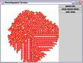
Fig. 2.3 shows the development of an
interesting agent taken from Phase One, shown at various times in the
development. An unfortunate point is that the majority of genotypes generate
trivial agents - nearly 80% of random samples. However, it will be shown that
selection quickly improves matters.
Fig. 2.2.
Development of an interesting agent.
We can now make some estimates
involving size: Firstly, we note that the maximum size of an agent
with numTel telomeres will be 2*(numTel+1)2 - this
is the size of a diamond with sides of length (numTel+1). Hence, an
agent with numTel = 6 will have a maximum phenotypic size of 98
cells; 882 cells for an agent with numTel = 20. In contrast, and
agent with numColours = 5 and numRules = 25 will have a
genotypic size of 175, regardless of phenotypic size.
The
complexity of the developmental process is O(numTel3*numRules).
3 Phase One: Application-Neutral Experiments
The evolution of cellular
automata is a notoriously difficult problem: the highly non-linear nature of
the space of CAs, as well as the unpredictability of the forecasting problem
[15], [13] makes the
prospect of the evolution of complex patterns using GAs seem grim. As we
have recognized the Bluenome model as a subset of the space of
two-dimensional CAs, it is not obvious that evolution is possible in any
reasonable measure of time. Phase One was a set of experiments utilizing an
array of fitness functions to determine which high-level axis could
potentially be evolved.
Phase one utilized a neutral view
of phenotypes - an organism was treated as an image, fitness function being
based on techniques from Image Processing. In all cases, grids of size
100x100 were used, and the agents were allowed to grow to fit the grid. A
genetic algorithm was used to evolve phenotypes, typically running for 100
generations with a population size of 30.
Successful experiments showed promising
results; Typically, highly fit population members were discovered prior to
generation 100, with steady increase in mean fitness. These fitness functions
included: selection for complexity, selection for similar but disconnected
regions, selection for highly distinctive regions, and selection for a
transport system (a minimal network of cells which neighbours as many cells in
the grid as possible).
An example of one such successful run
was the attempt to generate images of increasing complexity. Here, fitness was
a function of the size of the grown agent and the number of different cell
types included in the phenotype. By generation 100 a robust agent utilizing all
colours can be seen. Members of the population can be seen in Fig. 3.1. From
generation 100 of this same experiment, a visual continuity between population
members can be seen, as illustrated in Fig. 3.2
Fig. 3.1
Images from a Phase One experiment using
complexity as a fitness. Members are shown from generations 0, 10, 40 and
100.

Fig. 3.2
Visual examples of continuity from generation
100.
In addition to the
successful attempts at evolution, there were some unsuccessful examples as
well. One such example was the attempt to generate images using an entropy
function as fitness - that is, the attempt to grow images consisting of pure
noise. Although images near optimal fitness were found, following 300
generations of evolution, there was no significant increase in mean fitness
relative to generation zero. This is not surprising, given previous
arguments regarding developmental model's inherent structured growth. A
second example was the attempt to produce agents which terminate their own
growth prior to filling the grid;It
is for this reason that the numTel parameter is included, modeling
biological telomeres.
Fig. 3.3 shows a set of
exemplar members chosen from the various experiments. In all cases, these
members were found in less than 100 generations of evolution, utilizing
population sizes of less than 30.
Fig. 3.3
Exemplar members from Phase One experiments, identified by generating
fitness: (far left) maximal thin coverage; (left) disconnected
regions of similarity; (right) disconnected regions of similarity; (far right) highly distinctive regions.
Another interesting
result from Phase One was the attempt to re-grow a genotype in differing
environments. This attempt is illustrated in Fig. 3.4, where again visual
similarities may be seen most clearly, Additionally, under the fitness
used in the experiment (the complexity function), fitness was nearly
identical for each re-growth.
|
 
|

|
|

|
Fig. 3.4
Attempt to re-grow the same genotype is differing environments: (
top far left) original 100x100 grid; (right) 200x200 grid; (top
left) a square of non-interacting foreign cells; (bottom left)
100x200 grid.
|