Concordia University's DEC LAB: Research at the DEC LAB

In this experiment we used the dataset with 6 features in DB3. We randomly selected one feature from the dataset, and repeatedly added this features several times. We observed the accuracy of classification for GA-based FS, GA-based FW, as well as the unaided 1-NN classifier. The error estimation method is the same as that used in section 4.1.2 (above). 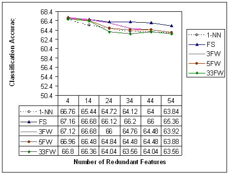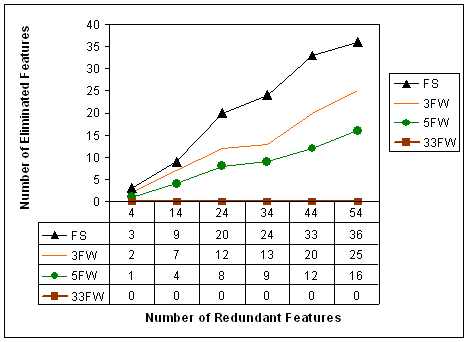The results of experimentation are shown in figures 4 and 5. Figure 4 shows the empirical relationship between the number of redundant features, present in the initial set of features, and the classification accuracy of the 1-NN classifier, acting alone, and with the help of GA-based feature selection/weighting. Figure 5 presents the relationship between the number of redundant features, and the number of features eliminated by FS and FW. A 1-NN, on its own does not eliminates any features, of course.

Figure 4: Classification Accuracy as a Function of the Number of Redundant Features

Figure 5: Number of Eliminated Features as a Function of the Number of Redundant Features

· Contrary to the case of irrelevant features, the classification accuracy of the 1-NN classifier degrades very gradually, as a function of the number of redundant features.

· In experiments with 4, 14 and 24 redundant features, FS classification accuracies are almost identical to those achieved by 3FW. However, for the same number of redundant features, the other feature weighting configurations returned classification accuracies that are worse, but only slightly.

· FS outperforms all other FW configurations in experiments where the number of redundant features is 34 or greater.

· As the number of weight levels increases, the classification accuracy of the feature weighting configurations slightly decreases.

· Although the difference in classification accuracy between FS and FW is not very large, the difference in terms of the number of eliminated features (shown in fig. 5) is significant.

· The difference in performance between FS and FW increases as the number of redundant features climbs. Finally, when the number of redundant features reaches 54, FS succeeds in eliminating 34 redundant features, 11 more than the best performing FW configuration (3FW).

Why does not the performance of the 1-NN classifier quickly degrade as the number of redundant features increases? The reason is that adding copies of an existing feature repeatedly to a set of features (to act as redundant features) is like giving that feature an added weight equal to the number of copies. For example, if a certain feature is added 20 times, this has the same effect as using this feature once, but multiplied by a weight of 20. On the other hand, completely irrelevant features add randomness and noise to the feature set, which cause higher classification error rates. Though the presence of redundant features in the training data might not significantly decrease the accuracy of the classification algorithm, it will certainly worsen the problem of dimensionality. Moreover, giving a certain feature higher weight simply because it was repeated is considered to be a random procedure (Wilson & Martinez, 1996).

In conclusion, the classification accuracy of a 1-NN classifier does not suffer greatly as a result of having a significant number of redundant features in the (original) feature set. However, due to the other problems associated with redundant features increased dimensionality (and hence computational cost), and arbitrariness of procedure, as well as slightly worse classification accuracies, it is recommended that a GA-based feature selection method be used to eliminate as many of the redundant features as possible. It is clear that the best suited feature selection/weighting methods for such a task are FS and 3FW. Which one is chosen depends on the need for real-valued weights vs. computational efficiency.

4.1.4 Performance of both FS and FW for Real-World and Regular Databases.

(Wettschereck et al., 1997) state that feature weighting (GA-based or not) is more suitable than feature selection for domains where features have a wide range of relevance. On the other hand, (Kohavi, Langley & Yun, 1997) show that increasing the number of weights above two rarely reduces classification error, for many real world datasets. They show that using only two weights (which is equivalent to feature selection) gives better results than increasing the set of weights. It is worth noting that the results of (Kohavi et al., 1997) are for small datasets (with less than 300 training samples), and use a best-first search algorithm. In contrast, we intend to compare feature selection to feature weighting using real-world and regular databases, with 1000+ training samples, and using GAs as a search method.

Presented here is a study of the classification accuracies achieved by the 1-NN classifier and the various GA-based feature selection (FS) and weighting (FW) configurations. The focus in this study is on assessing the true real-world performance of such configurations. This requires (a) that real-world databases (containing human-generated samples) are used, and (b) that any results achieved using training sets are checked against separate results obtained with new (unseen) validation sample sets. 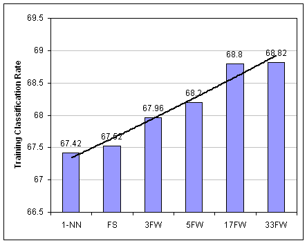The resultant accuracies for training and validation sample sets are displayed in figures 6 and 7. The database used for figures 6 and 7 was the 6 feature dataset in DB3. For figures 8 and 9, we used DB2. The error estimation method is the leave-one-out cross validation. It was applied to 1000 training samples. The best weights are tested using a separate set of 500 validation samples. To avoid bias, we randomly selected different training/validation sets for each experimental run. Each experiment is repeated 5 times, and the results reported are average values for those. The symbols on the X-axes indicate the following:

Figure 6: Training Classification Accuracies for the Various Feature Selection and Weighting Methods (using DB3)

Results show that classification accuracy is worst for the (unaided) 1-NN, but better for FS and FW. The trend line highlights the fact that the greater the number of weight levels the higher the training accuracy rate achieved. Finally, it appears that classification accuracy could not be improved much by increasing the number of weights beyond 17; the difference in classification accuracy between 17FW and 33FW is 0.02, which is insignificant.

Figure 7: Validation Classification Accuracies for the Various Feature Selection and Weighting Methods (using DB3)

Results show that classification accuracy is best for the (unaided) 1-NN and FS, but worse for FW. The trend line highlights the fact that the greater the number of weight levels the lower the validation accuracy rate achieved. Finally, it appears that classification accuracy cannot be further degraded by increasing the number of weights beyond 17; there is no difference in classification accuracy between 17FW and 33FW. These results are the opposite of those found in figure 6! This means that FW is returning good accuracy results for training data, but then returning bad results for validation data. Also, it is the performance of a classifier on validation data that truly reflects its (real-world) predictive capacity.

To verify these interesting results, we ran the same set of experiments on another database (DB2). This is to ensure that the above results are independent of the particular sample database used. The results are shown in figures 8 and 9. It emerges that the results of these experiments indeed confirm the results of figures 6 and 7.

Figure 8: Training Classification Accuracies for the Various Feature Selection and Weighting Methods (using DB2)

Figure 9: Validation Classification Accuracies for the Various Feature Selection and Weighting Methods (using DB2)

We believe the interesting disparity between training and validation results is due to over-fitting. FW allows for a finer-grain representation of the search space, but at the expense of an increased classification error rate. In other words, what we are faced with here is a typical bias vs. variance tradeoff (Geman, Bienenstock & Doursat, 1992). Classification error can be decomposed into two components, bias and variance. Bias measure how much the error estimation deviates from the true value, whereas the variance measures how much variability classification shows for different training samples. For example, assume that we have an infinite number of classifiers built from different training sets of the same size. The bias of a learning algorithm is the expected error of the combined classifiers on new data. The variance, on the other hand, is the expected error due to the particular training set used. Therefore using a small number of weights will increase the bias due to the lack of representation of the space. However, this will also reduce variance, which in turn reduces the possibility of over-fitting of data (Kohavi et al., 1997). In contrast, allowing many weights will reduce bias but will also increase variance, and the probability of over-fitting.

(Kohavi et al., 1997) also illustrate that increasing the number of weights above two hardly ever decreases classification errors. In their study they show that with 10 weights levels, FW fails to outperform FS on 11 real-world databases. They conclude that, "On many natural data sets, restricting the set of weights to only two alternatives-which is equivalent to feature subset selection-gives the best results". Though we used different search methods and larger datasets than those used by Kohavi et al., we get similar results and conclusions.

In addition, we should take into account that the databases we are using to report our results are handwritten character recognition databases. This means that there are many variants of letter shape, size, and generally, style. Also, different writers have different writing styles. For the letters of an alphabet, there are nearly an unlimited number of variations. Thus, feature weighting over-fits the training data by finding suitable weights, but these weights obtained do not generally represent the underlying distribution due to the large variance among the training samples.

On the other hand, other papers have shown that feature weighting using GAs yield a slightly better classification accuracy than feature selection for real-world databases. For example, (Punch et al., 1993) perform tests using binary and real-valued weights (with weights in [0,10]). Their database consisted of images of soil samples. Their results show that the error rates obtained using real-valued weights are better than those with binary weights. Also, (Komosinski & Krawiec, 2000) provide further evidence that feature weighting is somewhat better than selection when applied to a brain-tumor diagnoses system. Their results confirm that feature weighting (using weights in [0,9]) leads to somewhat better classification accuracy rates than just feature selection.

However, several points must be raised here. First, results reported in (Komosinski & Krawiec, 2000) are those of GA evaluation. No validation tests were done to test the resultant weights on separate data sets. In fact, (Kohavi & Sommerfield, 1995) have noticed this fact and states that separate holdout sets, which were never used during the feature selection/weighting, should be used in the final test of performance. Second, results reported by (Punch et al., 1993) were performed on validation samples, which were randomly drawn from the training samples. This also has the same biased effect on the results. Third, the improvement in classification accuracies mentioned in both papers for FW over FS is so little that it does not, in itself, provide final evidence that FW gives better results than FS on real datasets. Komosinski & Krawiec reports classification accuracies of 83.43

1.93 and 77.83

2.03 (for two datasets) for FW, vs. accuracies of 80

1.22 and 75.7

1.64 for FS. While Punch et al. reports a classification error rate for FW of 0.83% and 2% for training and testing respectively, those of FS were 1.66 and 3.2% for training and testing.

In conclusion, despite the fact that feature weighting has the best training classification accuracies, feature selection is better in generalization, and hence more suited to real-world applications (in which most data is new). This is because FW overfits the training data, losing generalizability in the process. Therefore, it is advisable to use 2 (FS) or 3 (3FW) weight levels at most, as (Kohavi et al., 1997) recommend.

4.2 Feature Selection Evaluation Results

The following are two empirical studies that study the effectiveness of GA-based feature selection (GFS) with respect to (a) finding a provably optimal set of features, and (b) doing so within an acceptable time frame, for off-line applications (e.g., pre-release optimization of character recognition software).

4.2.1 Convergence of FS to an Optimal or Near-Optimal Set of Features

In the context of feature selection, several comparative studies involving Genetic Algorithms and other search and optimization algorithms are available. (Vafaie & De Jong, 1993) show that GA outperforms sequential backward selection in robustness. They demonstrate that genetic algorithms improve robustness of feature selection without a major increase in computational complexity. Moreover, (Handels et al., 1999) compare a number of feature selection methods: Genetic Algorithms other heuristic searches, and 'greedy' methods (forward and backward searches). Their domain of application is diagnosis of skin tumors. The best classification accuracy is obtained by the GA. (Estevez & Fernandez, 1999) perform a comparison between Genetic Algorithms, statistical methods and the leave-one-feature-out approach, all in the context of classifying wood board defects. The GA gives the best performance among the three techniques, but at the expense of high computational complexity. (Kudo & Sklansky, 2000) provide a recent comparison of different feature selection algorithms (including GAs) for large feature spaces. The authors conclude that Genetic Algorithms are more suited than other feature selection algorithms for problems with more than 50 features. However, for small (0-19 features) and medium (20-49) cardinality, GAs though useful, are too slow to justify their use.

It is clear from the literature that several studies exist comparing GA with other feature selection search algorithms, so it not our intention to repeat such work. However, there is a need to determine whether or not GFS does indeed return optimal or near-optimal feature sub-sets. This necessitates an exhaustive search of the features space in order to find one or more bona fide optimum feature sub-set. These can then be used to assess (with certainty) the optimality of the best GFS-generated feature sub-sets.

For the experiments in sections 4.2.1 and 4.2.2, we used a single training/testing set of size 1000 and 500, respectively. The numbers of features used in the searches are 8, 10, 12, 14, 16, and 18. We used features from more than one dataset in DB3 for that purpose. There is no need to have a separate validation set since our objective here is to evaluate optimal performance, and not test generalizability.

Number of Features	Best Exhaustive (classification rate)	Best GA (classification rate)	Average GA (for 5 runs)
8	74	74	74
10	75.2	75.2	75.2
12	77.2	77.2	77.04
14	79	79	78.56
16	79.2	79	78.28
18	79.4	79.4	78.92

Table 3: Best Classification Accuracy Rates Achieved by GA and Exhaustive Search

The results presented in table 3 compare the best and average accuracy rates achieved via GA-based feature selection (FS) with the optimal accuracy rate found via an exhaustive search of the entire feature space.

Comparing the numbers in the best GA column with the numbers in the best exhaustive column exhibits the success of the GA as a feature set optimizer. In every case but one (when the number of features is 16), the best accuracy achieved by the GA was identical to that found an exhaustive search of the feature space. Furthermore, the fact that the worst average GA value is less than 0.8 of a percentage point away from the optimal value means that the GA was consistently able to return optimal or near-optimal values of accuracy. Hence, GA-based feature selection consistently converges to an optimal or near-optimal set of features.

4.2.2 Convergence of FS to an Optimal or Near-Optimal Set of Features within an Acceptable Number of Generations.

In general, the run time for the GA is proportional to the number of features, number of generations and size of the population (Kudo & Sklansky, 2000). Moreover, the time complexity of the nearest neighbour classifier is proportional to (

x d), where t is the number of training instances and d is the number of features used. So a GA that is applied in a wrapper configuration to a nearest neighbour classifier spend most of its time running the nearest neighbour classifier (Brill, Brown & Martin, 1992). Below, we list those factors that affect the time complexity of our GFS or GFW:

In this evaluation, we will investigate the relationship between the number of features (in the original set) and the number of generations required to reach an optimal or near-optimal sub-set. We will do that while keeping the two other factors (i.e. population size and number of training instances) constant.

The results of experimentation are shown in table 4. The second column of table 4 shows the best (i.e. optimal) classification accuracy rates attained using an exhaustive search, whereas the third column displays the duration of that search. The fourth column contains the best results achieved via a GA-based search, while the fifth column contains the time it took the GA to attain those values.

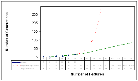
Figure 10 below displays the relationship between the numbers of generations needed to reach

optimal or sub-optimal values with a GA, and the number of features in the original set. The tiny triangles represent actual data from table 4 (above). There are also two curves in figure 10. The solid line represents a best-fit piece-wise linear curve that fits to, and extrapolates, the data points. The extrapolated segment of this curve (beyond 18 features) represents the most optimistic projection of GA run time duration. The dotted line represents an exponential curve that fits to, and extrapolates, the same data points. The extrapolated segment of this curve (again, beyond 18 features) represents the most pessimistic projection of GA run time duration. The reason for use of extrapolation is the obviously impossible amount of time required to run exhaustive searches of large feature spaces using a single-processor computer. In any case, one can safely conclude that the time needed for a GA-based search is bound, on the lower side by the (optimistic) best-fit curve, and on the upper side, by the (pessimistic) exponential curve.

Figure 10: Number of Generations to Convergence as a Function of Number of Features

Using exponential extrapolation, the number of generations expected for 60 features is 10585, while it is only 89 for linear extrapolation. The true value should be something in between. If we assume that the true value is midway between 89 and 10585 (which is 5337), then running the GA will be computationally expensive. In such cases, using methods of parallel GA, such as DVeGA (Moser, 1999), becomes necessary. Also, the authors are currently involved in the construction of a 10-processor dedicated Linux-PC cluster, which allows for genuine implementations of parallel GA architectures, including the one just mentioned. This is important, since the relative value of GA-based techniques is most pronounced when the search (e.g. feature) spaces involved are quite large.

We conclude that GA-based feature selection is a reliable method of locating optimal or near-optimal feature sub-sets. These techniques also save time, relative to exhaustive searches. However, their effective use in large feature spaces is dependant upon the invention of specialized feature selection/weighting methods (e.g., DveGa) or/and the availability of parallel processors.

4.1.3 Performance of both FS and FW in the presence of redundant features.

4.1.4 Performance of both FS and FW for Real-World and Regular Databases.

4.2 Feature Selection Evaluation Results

4.2.1 Convergence of FS to an Optimal or Near-Optimal Set of Features

4.2.2 Convergence of FS to an Optimal or Near-Optimal Set of Features within an Acceptable Number of Generations.