|
3. The Multi-Population Genetic Algorithm
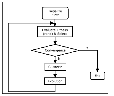
The overall operation of the multi-population GA is
presented graphically in Fig. 2.

Initially, a single population is created by
creating a number of chromosomes who's genes (see section 3.2) are
randomly selected from the set of foreground pixels in the image.
The population is then ranked in terms of both similarity and
distance and searched for good candidates- if any. If, by
chance, all the ellipses in the image are included in the first
generation, the program terminates. Otherwise, a clustering
technique is used to divide the chromosomes into a number of
clusters (or subpopulations). From that moment on, all the
subpopulations are evolved, in parallel. If one of the
subpopulations converges on an optimal or a suboptimal chromosome,
then that whole subpopulation and the corresponding ellipse (in the
image) are removed. This has the positive side effect of
accelerating the search process, since the rest of the
subpopulations will have one less ellipse to search for. The
program, as a whole, terminates when all (full and partial) ellipses
are found, or when a pre-set maximum number of generations is
reached.
The following sections (3.1 - 3.6) detail the key
steps of the MPGA algorithm, starting with an introduction to
elliptic geometry and concluding with clustering.
3.1 Ellipse Geometry
Chromosomes, in the MPGA, are no more than candidate
ellipses, and hence understanding the geometry of ellipses is
essential to understanding chromosomal representation, within the
MPGA. The ellipse equation can be written as:

Assuming we have five distinct points belonging to
the perimeter of an ellipse, we can solve 5 linear equations,
simultaneously, for
a, h, b, g, f.
One efficient numerical technique for solving linear equations is
the LU Decomposition algorithm [17].
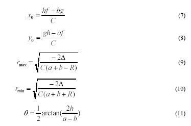
The geometric parameters for the ellipse are given
accordingly [14]:

where,

Again, the LU Decomposition algorithm [17] is used
to compute
Δ
efficiently.
3.2 Representation and Initialization
We represent chromosomes (using Roth et al.
approach [15]) with a minimal set of points on the shape's
perimeters. Since we need 5 points, each chromosome contains 5
genes. And, since each gene (point) has both horizontal and vertical
coordinates, the total number of numbers in a chromosome comes to
10.
There are, in the literature, alternative ways of
chromosomal representation of ellipses. For example, Mainzer [11,
12] represents an ellipse with a different set of five parameters
(see Fig. 3): a and b, which are the dimensions of the
long and short axes of an ellipse, respectively; x0 and y0,
which are the X and Y coordinates of the center; and finally
θ,
the angle the long axis makes with the X-axis the (or the rotation
angle).
In contrast, Lutton et al. [10] encode an
ellipse using the center O; a point on its perimeter P;
and rotation angle a. Lutton et al. (and so could
Mainzer) claim that their representation is preferable to Roth's
representation of ellipses, since Roth's chromosomes allow for
redundancy, and their chromosomes do not. This is so, since many of
Roth's chromosomes (which are 5-tuples of points) could belong to
the same ellipse.
Nevertheless, the encoding of ellipses via
their geometric parameters is also problematic. These techniques
provide no guarantee that the resulting candidate ellipses will
actually contain any point from any of the actual ellipses in the
target image. Using these techniques amounts to blindly placing
ellipses at randomly selected locations within the image, in the
hope that some of them will partially overlap some actual ellipses
in the image. Hence, such algorithms spend a long (if not most of
their) time evaluating the fitnesses of many chromosomes
representing useless candidate ellipses.
Therefore, we choose to encode a chromosome with a
set of 5 points, as Roth et al. did [15]. The redundancy
problems identified by Lutton et al. can be avoided by
disallowing identical chromosomes in the population. Two
chromosomes are identical if their phenotypes (geometric
parameters), and not genotypes (sets of points), are identical.
The MPGA algorithm creates an initial population of
between 30 and 100 chromosomes, depending on the
complexity of the target image. The five points
comprising each new chromosome are selected, at random, from the
set of foreground (or black) pixels in the target
image.
3.3 Fitness Evaluation
Most of the reported work in this area, such as [10,
11, and 12], evaluates the fitness of a candidate ellipse
(chromosome) by, essentially, counting the number of black pixels in
the target image which coincide with the perimeter of the candidate
ellipse. These black pixels may or may not belong to actual ellipses
in the image. However, if many pixels in the actual image match a
candidate ellipse then it is highly probable that theses pixels form
part of an actual ellipse in the image.
To enhance the robustness of the matching function,
Mainzer [11, 12] distinguishes pixels lying near the perimeter of a
candidate (ideal) ellipse from those far from it, and assigns a
penalty to the latter. Mainzer defines fitness S of a given
candidate ellipse as:

E(x+i, y+j) is a function that returns 1 if there
exists a foreground pixel (x+i, y+j) coincident with,
or close to a pixel (x,y) on the candidate ellipse. Otherwise
the function returns 0. i and j are the horizontal and
vertical displacements, respectively, between the two pixels.
Finally, d is a constant (determined by the nature of the
image). If there exists points in the image that exactly (i.e. i
= 0 and j = 0) match every point in the candidate ellipse
then this candidate ellipse will receive the maximum fitness of 1.
In [10] Lutton et al. use a grey-level
"distance image", where each pixel's grey value indicates its
distance to the nearest contour point. This distance image is
computed from the original image using two morphological masks. Like
Mainzer, they also punish points not exactly on the perimeter of a
candidate ellipse, using a displacement factor. However, the
construction of the distance image requires serious extra storage.
And the manual tuning of the two distance parameters in the mask
requires extra preparatory work, before the algorithm can be used.
Lutton et al. [10] also introduced another
fitness term that counts effective contour pixels "to favor bigger
primitives [or shapes]". However, bigger shapes are not necessarily
better ones; and the extent to which an actual pattern matches a
candidate shape has nothing to with the patterns absolute length or
size.

Neither of the measures of fitness discussed above
satisfy our requirements. Our aim is to detect full as well as
partial multiple ellipses with varying types and degrees of
imperfections. Fig. 4 provides concrete examples of such shapes,
where ellipse no. 3 shows a partial ellipse, and ellipse no. 2 is an
ellipse with an irregular outline. These two measures of fitness are
defined formally below. Therefore, we propose that the fitness of a
given candidate ellipse is measured in terms of both (a)
Similarity: how well the candidate's perimeter matches (or not)
the perimeter of an ideal complete ellipse; and (b) Distance:
how close or far is the perimeter (or part of it) to the perimeter
of an ideal ellipse (or part of it).
A. Similarity (S) is defined as:

The value of S belongs to [0, 1], with 1
indicating a perfect match and 0 no match at all. For a given point
(x,y) on a candidate ellipse, the term E(x+i, y+j) returns 1
if there is a point in the target image that coincides with, or is
close to (x,y); otherwise E(x+i, y+j) returns 0.
The terms i and j represent the
horizontal and vertical displacements, respectively, between a point
on the ideal ellipse and the corresponding actual point in the
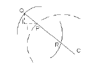
image. Fig. 5 shows how an actual point (Q) is determined and how
the distance between this point and the corresponding point (P) on
the candidate ellipse is computed.

Fig. 5
Matching of a Candidate Ellipse, Point by Point, to Potential Actual
Ellipses in an Image
In Fig. 5, the dashed arc belongs to an ideal
template with centre C. The solid arcs belong to actual (full or
partial) ellipses in the image. If P does not coincide with any
point in the image (in which case, P=Q), then a line is extended
from C passing through P, and radiating outward. A fast search,
based on Brensenham's algorithm [6], is initiated along this line
until a point (Q) on some pattern is found. This point is the
corresponding actual point, and the horizontal and vertical
displacements between it (Q) and P represent the i and j
terms, respectively, used in the computation of distance dij.

#total is the total number of pixels on the
candidate ellipse's perimeter.
To compute S efficiently, we further assume
that the ideal template is centered at the origin of coordinates
with a horizontally aligned long axis (Fig. 6).

Fig. 6
2D Geometric Transformation of Ellipse
A classic midpoint ellipse algorithm [6] is then
used to traverse the perimeter of this candidate ellipse. This
algorithm uses favours integer computation, and it only computes a
quarter of the ellipse's perimeter. All the other points in the
remaining 3 quadrants are obtained from symmetry. Each computed
pixel is matched to its "actual" ideal position using:

(x, y) are the original coordinates
and (xT ,yT ) are the transformed coordinates.
Finally, the term E(x+i, y+j) is replaced by ET(x+i, y+j)
, giving us the final form of the similarity equation:

B. Distance (D) is defined as:

D ranges from [0, ∞) The term di,j is
defined in (17) above. #eff is the total number of points on
the actual ellipse that were successfully matched with points on the
ideal ellipse. One reason for using #eff here instead
of #total is that actual ellipses may be missing parts of
their perimeter, i.e. there may be partial or highly irregular
ellipses in an image.
Similarity is the main measure, since it is directly
observable by the human eye. However, distance is particularly
important for cases where multiple ellipses are present in the
image, and especially when complete ellipses (with high similarity)
as well as imperfect ellipses (with relatively low similarity)
exist. We aim to seek those candidates with good similarity and
small distance, or those with acceptable similarity but
excellent distance. Obviously if, for a given candidate ellipse,
both of these measures return bad values, then this candidate can be
reasonably ignored as noise.
Again, Fig. 4 shows an example of an image with
perfect and imperfect ellipses. Table 1 lists the fitness values (in
terms of both similarity and distance) for the best three candidate
ellipses produced by an MPGA run. There will exist in the population
many other candidate ellipses, but all the fit ones will eventually
cluster around these three highly fit candidates.

Table 1
Fitness of Ellipses in Fig. 4
Without distance, it is highly possible that the
population will converge towards ellipse 1, while ignoring the other
two (very real) ellipses in the rest of the image. However, with
distance included, candidate ellipses converging on ellipses 2 and 3
will be ranked highly in terms of distance. Since the ellipses
converging towards these two ellipses will have acceptable
similarity but excellent distance, this will result in a
reasonable clustering (and hence subdivision) of the population,
instead of complete domination by ellipse 1 candidates.
In MPGA, fitness is computed in the following
manner: the 10 numbers of each chromosomes are substituted in
equations (7-14). If the equations fail to produce a solution then
this chromosome does not represent any kind of ellipse. Hence, this
chromosome is assigned the minimum fitness of 0. If the equations
produce a solution, then equations (19-20) are used to compute the
similarity and distance of this chromosome. These two values
together represent the fitness of the evaluated chromosome.
Page 1, Page 2,
Page 3,
Page 4
|