|
3.4 Termination Conditions
MPGA starts its run with a single population.
However, it usually splits it into a number of evolving
subpopulations. The termination of the evolution of any one of these
subpopulations occurs independently of the termination of the rest
of the subpopulations. A subpopulation terminates if any one of the
following conditions is fulfilled:
Condition 1: Optimal Convergence. If there
exists one (or more) "optimal" chromosomes. An optimal chromosome is
one with S > 0.95 and D < 10;
Condition 2: Sub-optimal Convergence. If
there exists one (or more) "good" chromosomes and 30 generations
have passed without the evolution of an optimal chromosome. A good
chromosome is one with S > 0.7 and D < 10;
Condition 3: Stagnation. 500 generations have
passed without the fulfillment of either Condition 1 or 2.
Also, a subpopulation is effectively terminated when
it is merged with another subpopulation (see section 3.5).
3.5 Clustering: Migration, Splitting and Merging
A subpopulation is called a cluster. The
centre of a cluster is the chromosome with the greatest similarity.
If more than one exists then the one with the least distance is
declared the centre.
In the MPGA algorithm, the algorithm starts with a
single population (or cluster) in which individuals are ranked in
terms of both similarity and distance. The initial
single population, and later subpopulations, are manipulated through
a clustering process. This process involves Migration, Splitting and
Merger (explained below).
In each subpopulation, all good chromosomes (S>0.7
and D<10) are either kept in their own cluster or placed into a
different existing or newly-created cluster. All not-good
chromosomes are simply left in their own cluster (and are eventually
eliminated be selection- see section 3.6).
The Euclidean distance ED between a good
chromosome and the various existing cluster centers determines
whether this chromosomes remains in its own cluster or moves. ED
is computed as follows: given two sets of ellipse parameters (a1,
b1, x1, y1, ω1) and (a2, b2, x2, y2, ω2):
(ai, bi) is the long and short axis, (xi,
yi) is the center and ωi is the orientation. When a
chromosome migrates from subpopulation A to subpopulation B, it
replaces the weakest chromosome in the latter, and the vacancy in
the former is filled by the processes of evolution (see section
3.6).
A. Migration. If the Euclidean distance
between a chromosome and its own cluster centre is lower than a
pre-defined threshold t1 then this chromosome is moved to
another cluster. To determine which one, the ED between this
chromosome and every other cluster center is measured. If one or
more cluster centers is closer to it than t1 then the
chromosome moves (migrates) to the cluster with the closest centre
to it.
B. Splitting. If the algorithm is unable to
find a cluster (with a centre) sufficiently close to a migrating
chromosome, then a new cluster is created around this chromosome.
This action is called splitting.
C. Merging. An empirically-derived threshold σd is used to define the minimum allowable Euclidean distance
between any two different cluster centers. As two different clusters
may evolve toward a single (local or global optimum), any two
clusters with centers closer to each other than σd are merged. This
is done by taking the fittest 50% (in terms of similarity) of the
chromosomes in each cluster and placing them in the new merged
cluster. This action is called merging.
All clusters are checked periodically (every 30
generations), to see whether some of them could be merged. Merging
is barred for the first 50 generations, and (as stated) is only
possible after each periodic check. This is so because early or/and
frequent mergers would greatly reduce the diversity of the whole
population.
Hence, through the three processes of migration,
splitting and merger, clustering works to maintain a number of
subpopulations that are independently evolved towards local and
global optima. Evolution is explained in the next section.
3.6 Evolution: Selection and Diversification
Evolution proceeds mainly via Selection and
Diversification. Selection eliminates those chromosomes in the
population that are not very fit, focusing the search on promising
areas of the fitness surface. On the other hand, diversity is
achieved via crossover and mutation, which together serve to direct
the search towards new and potentially promising areas. In MPGA,
selection is realized using Elitism and Fitness Proportional
Selection.
Diversification is realized via Crossover and
Mutation.
During evolution of a subpopulation, elitism copies
the fittest 15% of the current generation (by similarity) into the
next generation, without modification. Following that, two
chromosomes are selected from the whole current population. The
probability of selecting a chromosome is proportional to its
relative fitness (similarity). The two chromosomes are crossed-over,
with probability 0.6. The result, whether it is two new chromosomes
or the original parent chromosomes, are mutated (on a bit-wise
basis) with probability 0.1. This process of selection and
crossovermutation continues until the next generation is complete.
As stated, we use constant size subpopulations of between 30 and 100
chromosomes.
Finally, every new chromosome introduced into the
next generation is tested to see if it is a good chromosome or not
(S>0.7, D< 10); if it is not then it is left in the same
subpopulation. If however it proves to be a good chromosome then it
is tested for migration-splitting, and is then either kept in its
current subpopulation or moved to another existing or new
subpopulation (see section 3.5).
In MPGA, Crossover and Mutation are special
operations designed specifically for shape detection applications.
We describe them in detail below, starting with crossover.
Given the fact that (a) the overall population is
divided into a number of subpopulations, each effectively clustering
around an ellipse in the image; and (b) each chromosome is defined
by a set of points on the perimeter of an ellipse, we can assert
that simple single point crossover is an effective method of
crossover for our application. A pivot is selected at random, and
the parent chromosomes' genes on either side of the pivot are
swapped to create the offspring. See Fig. 7.
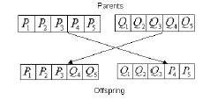
Fig. 7
Result of Crossing-Over Two Chromosomes: Genotypic View
The effect of the crossover operation, on the actual
ellipses represented by the chromosomes, is shown in Fig. 8.

Fig. 8
Result of Crossing-Over
Two Chromosomes: Phenotypic View
For mutation, we define a new mutation operator,
configured specifically for our application. First a gene (or point)
is randomly selected from the chromosome that we intend to mutate.
As shown in Fig. 8, this point acts as the starting point for a path
(r) that traverses the perimeter of a pattern, until a
(pre-set) maximum number of points is traversed, or an end- or
intersection point is reached. If r > 10, the remaining genes
(points) are also picked, at random, from this path. As long as the
starting point lies on a promising candidate ellipse, it is highly
possible that the other points will do so as well. This method of
mutation greatly enhances the possibility of mutating a given
chromosome into a better one.
Fig. 9 illustrates the mutation process. The
original genes are P1, P2, P3, P4, and P5. The starting point, P1 is
selected and path r is traversed. The other new genes, Q2,
Q3, Q4, and Q5 are randomly selected from path r, and copied
into the mutated chromosome. Hence, the new chromosome becomes
(P1Q2Q3Q4Q5).

Fig. 9
Mutation Operation
Hence, evolution hand-in-hand with clustering (which
mainly precedes but also acts during evolution) direct the various
subpopulations to local and global optima centered on the various
ellipses in the target image.
4. Experimental Results and Analysis
This section compares the performance of the MPGA,
SGA and RHT algorithms, using synthetic and real-world images. To
carry out a fair comparison between these three different
algorithms, we use (a) the same method for computing fitness, in
terms of similarity and distance (described in section 3.4), and (b)
the same numerical technique for computing the geometric parameters
of an ellipse (see section 3.1). This neutralizes any advantages
that may be gained via using more efficient methods, which reduce
dimensionality or utilize symmetry [5, 7, 9, 13].
All our experiments were run on an Intel Xeon 2.66
GHz w/ 512 KB of cache, 512 MB DDR RAM and running Red Hat Linux
8.0.3.2-7.
We have two main categories of test data, which are
synthetic images and real world images. Accuracy here, is defined as
the ratio of correctly detected ellipses, in relation to the total
number of ellipses actually present in the target image. If over
detection occurs, then that is reflected in the false positive (fp)
statistics.
4.1 Synthetic Images
The synthetic images are comprised of two sets, set
A and set B. Set A is partitioned into 7 collections of 50 images
each (totaling 350 images). These collections are used to test the
algorithms' performance on images with different numbers of
ellipses. Hence, the first collection contains 50 images of single
ellipses, the second collection contains images of two ellipses, and
so on. The final collection contains 50 images of 7 ellipses. Set B,
on the other hand, is used to test the algorithms' performance on
noisy images. Hence, this set is made of 5 collections of 50 images
each (totaling 250 images). The first, second, third, fourth and
fifth collections contain images with 0%, 0.5%, 1%, 3% and 5%
salt-and-pepper noise, respectively.
The ellipses in the synthetic image database are not
all full and perfectly formed ellipses; we make sure that some images in both sets have at least 1 partial or
deformed ellipse. A typical example is presented in Fig. 10. In this figure there are 6 ellipses, 2 of which are
malformed. The figure also shows the results, in terms of detected
ellipses, of applying MPGA, RHT and SGA to this image.

Fig. 10
A Typical Image with Multiple Ellipses: Detected Ellipses Overlaid
in Thick Grey Line (a) Original Image (b) Ellipses Detected by MPGA
(c) Ellipses Detected by RHT (d) Ellipses Detected by SGA

Table 2
Parameter Values for Ellipses Detected in Fig. 10
As seen in Fig. 10 (c), RHT misses the smallest
ellipse and the partial ellipse since (in line with equation (1))
the probability of locating it is smaller than the
probability of locating the other larger ellipses. The fitness
values shown in Table 2 are those of similarity and not distance
(or some combination of the two) because: (a) similarity is the only measure/factor of fitness used by all these
three algorithms, and (b) similarity is more intuitive than any combination of measures, since it closely
corresponds to the human conception of similarity between shapes.
In reference to Table 2, MPGA returns better fitness
values than RHT, for ellipses 1, 2, 3 and 4. This is because MPGA, via evolution, executes an iterative and
parallel search, focused at different localities of the of the
search space, while the RHT carries out a one-shot blind
search through the whole space.
Fig. 11 contrasts the performance of the three
algorithms in terms of accuracy as well as average CPU running time. Fig. 11(a) shows that the accuracy of SGA
decreases dramatically as the number of ellipses increase.
Similarly, the accuracy of RHT also decreases gradually from
100% for one ellipse to approximately 80% for seven ellipses. In contrast, MPGA outperforms the other two algorithms
by maintaining an almost perfect level of detection accuracy, and slightly dipping to around 98%, for images with
seven ellipses.

Fig. 11
Comparing the Performance of RHT, SGA and MPGA when Detecting
Multiple Ellipses in an Image (a) Accuracy vs. Number of Ellipses
(b) CPU Time vs. Number of Ellipses
Fig. 11(b) demonstrates the clear advantage that
MPGA has over both RHT and GAS in regards to speed time. It graphs
the amount of CPU time utilized (on average) by the various
algorithms for the detection of images with 1-7 ellipses. There is
almost no difference in speed for images with 4 or less ellipses.
However, for 5 or more ellipses, MPGA realizes a clear and widening
gap in speed.
Fig. 12(a) shows a typical image with 5%
pepper-and-salt noise. Ellipses detected by MPGA are shown in Fig.
12(b)
Fig. 12
A Typical Noisy Image with %5 Salt & Pepper Noise: Detected Ellipses
Overlaid in Thick Grey Line (a) Original Image (b) Ellipses Detected
by MPGA (c) Ellipses Detected by RHT (d) Ellipses Detected by SGA
Table 3
Parameter Values Ellipses Detected in Fig. 12
Generally, RHT is more liable to false positives
(i.e. the detection of non-existing ellipses). Fig. 12(c)
demonstrates that.
Fig. 13 shows the performance of these algorithms on
noisy images. Again, MPGA shows considerable robustness in the
presence of salt-and-pepper noise, while simultaneously operating
faster than the other two algorithms.

Fig. 13
Comparing the Performance of
RHT, SGA and MPGA when Detecting Ellipses in Noisy Images (a)
Accuracy vs. Ratio of Noise in Image (b) CPU Time vs. Ratio of Noise
in Image
Many false positives are observed for RHT with high
noise, as Fig. 14 shows. This fact further fortifies our claim (in
section 1) that RHT searches the space and accumulates votes
blindly. Therefore non-existing ellipses may get enough votes in
highly noisy images, as is the case in Fig. 14.

Fig. 14
False positives for different noise level
Page 1,
Page 2, Page 3, Page 4
|